What is FIV3 (Filtered Incremental Velocity)? A Next-Generation Intensity Measure Explained
What is FIV3?
FIV3(T), filtered incremental velocity, is a next-generation ground motion intensity measure, proposed by Dávalos and Miranda (2019), that measures the largest velocity increments a ground motion delivers over time windows tied to a structure's period T.
An intensity measure (IM) is the single number used to describe how strong the ground shaking is, such as peak ground acceleration (PGA) or spectral acceleration at a period T, Sa(T). Fragility and vulnerability models are conditioned on an IM, so the choice of IM decides how much of a structure's response the model can explain.
Sa(T) is the workhorse of practice, but it describes the shaking at only one period. A structure that yields softens, its period lengthens, and higher modes come into play, so the shaking at other periods matters too. Next-generation IMs, such as average spectral acceleration, Saavg(T) (Baker and Cornell 2006), and FIV3(T), are designed to capture this, and have been shown to predict structural response much better. FIV3 differs from Saavg(T) in one important way: it does not use a response spectrum at all. It works directly on the acceleration trace of the record.
How is FIV3 computed?
FIV3 is computed in three steps.
- Filter. The acceleration record is low-pass filtered to remove the high frequencies that do little damage to a structure of period T.
- Integrate over sliding windows. The filtered acceleration is integrated over sliding windows of length 0.7T. Since the integral of acceleration is velocity, this gives the velocity increment that the ground delivers within each window, as a function of the window's start time.
- Sum the largest increments. FIV3 is the larger of the sum of the three largest peaks and the sum of the three largest troughs of that incremental velocity history.
In equation form, with the filtered ground acceleration and :
The result is a velocity, and the djura package reports it in cm/s. The figure below shows the two steps for a real record: the filtered acceleration, and the windowed incremental velocity with its three largest peaks and troughs.
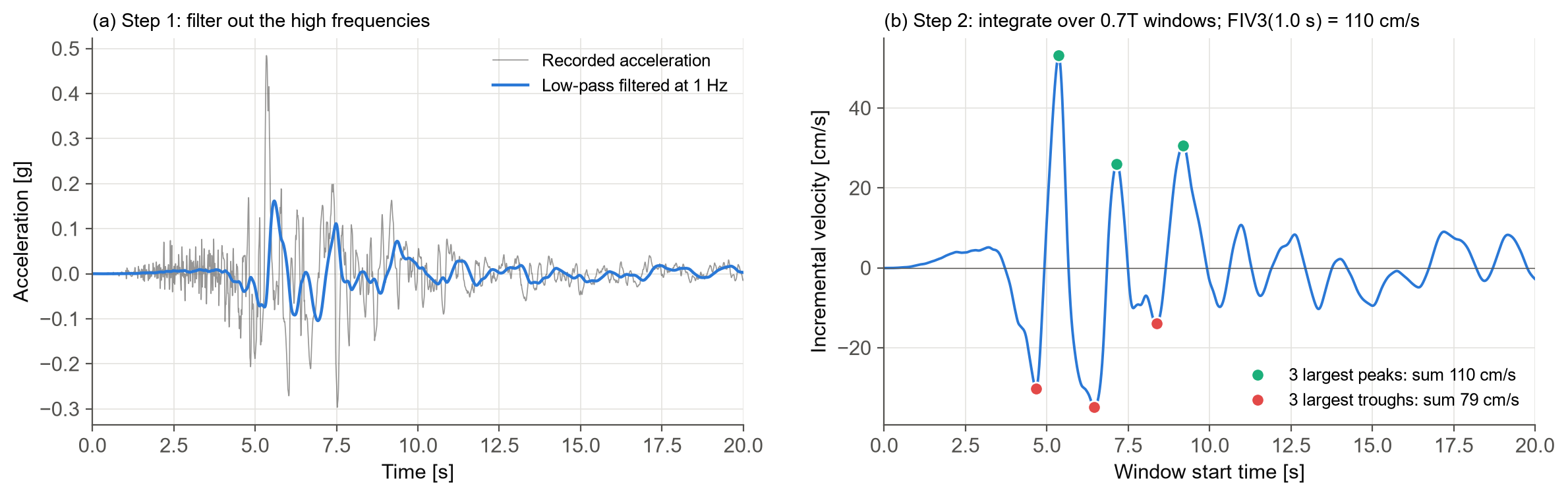
For this record, FIV3(1.0 s) is 110 cm/s. The window length, the filter cut-off and causal or acausal filtering are all parameters of the definition, and can be changed in the djura implementation.
Why does FIV3 predict structural response so well?
FIV3 responds to the large, coherent velocity increments that push a structure towards collapse, which is why it performs so well for collapse prediction. Sa(T) records the peak response of an elastic oscillator, which can be governed by a single short spike in the record. A velocity increment sustained over a window comparable to the structure's period is closer to what drives a yielding structure to large displacements.
Because the low-pass filter strips out high frequencies, FIV3 also does not react to the short, high-frequency peaks that often set PGA.
What does efficiency mean in practice?
An IM is called efficient when it explains a structure's response well, so that the response varies little among ground motions with the same IM value. In a fragility model, this shows up directly as the dispersion: a steep fragility curve with a small dispersion means an efficient IM.
In the study of O'Reilly, Ozsarac and Shahnazaryan (2026), the same structure (a single-degree-of-freedom system with a period of 1.0 s) was analysed with multiple stripe analysis, and its fragility functions were fitted directly in several IMs. For the same damage state:
| Intensity measure | Fragility dispersion |
|---|---|
| PGA | 0.72 |
| Sa(1.0 s) | 0.46 |
| Saavg3(1.0 s) | 0.17 |
| FIV3(1.0 s) | 0.17 |
FIV3(1.0 s) and Saavg3(1.0 s) both explain this structure's response far better than Sa at the structure's own period, and PGA explains it worst of all. These numbers apply to one structure at one site; they illustrate the pattern rather than a universal value.
Why is FIV3 a "universal donor"?
Efficiency matters well beyond the fragility model itself. When fragility or vulnerability models built on different IMs need to be used together in a regional risk model, they are often converted between intensity measures so that one ground motion field serves them all.
The main finding of that study is that conversion only works from a more efficient IM to a less efficient one. The unexplained spread in a model built on an inefficient IM is information that has already been lost, and no conversion can put it back. Across all the IM pairs tested:
- A model built on FIV3(T) converts reasonably to every target IM. FIV3 at different periods also converts easily between its own definitions, because it is nearly period-independent.
- A model built on PGA cannot be converted to anything better, although other IMs convert into PGA quite well.
Borrowing the terminology of blood transfusion: PGA is a universal receiver, and FIV3(T) is a universal donor. The same holds for losses. A vulnerability model in Sa(1.0 s) converted to FIV3(1.0 s) gave an average annual loss within 5% of the reference, and models built on FIV3(T) stayed within about 10% on average for targets other than PGA.
The practical advice from the study follows directly: build new fragility and vulnerability models on efficient, next-generation IMs such as Saavg(T) or FIV3(T), so that they can be reused and converted by people who did not build them. For a broader comparison of the classic IMs, see PGA versus spectral acceleration for fragility analysis, and for the basics of the models themselves, what a fragility curve is.
What do you need to use FIV3 in a risk assessment?
An IM is only useful in a probabilistic assessment if three things exist for it:
- A way to compute it from records. The
signal_processingmodule of the open-source djura Python package computes FIV3 for a single component or for any RotDxx percentile of a horizontal pair. FIV3 is computed in every direction before the percentile is taken, rather than derived from a rotated spectrum. - A ground motion model, to predict its distribution for an earthquake scenario and build hazard curves. The artificial neural network-based model of Aristeidou et al. (2024) predicts next-generation IMs, including FIV3.
- Correlation models, to relate FIV3 to other IMs. These are needed for conditional record selection and for IM conversion. Aristeidou et al. (2025) provide correlation models for next-generation amplitude and cumulative IMs.
With these in place, FIV3 can be used like any other IM. The Djura record selector (Shahnazaryan et al. 2025) accepts FIV3 as an IM in its generalised conditional spectrum record selection and in its scenario-based record selection.
Computing FIV3 in Python
The code below computes FIV3(1.0 s) for one component and the RotD50 value for a horizontal pair. The full walkthrough, with the record used here, is in our post on ground motion signal processing in Python.
from djura import signal_processing as sig

dt, npts, desc, t, acc1 = sig.read_nga("RSN179_IMPVALL.H_H-E04140.AT2")
_, _, _, _, acc2 = sig.read_nga("RSN179_IMPVALL.H_H-E04230.AT2")

h1 = sig.Component(acc1, dt, unit="g")
h1.fiv3([1.0])                       # 110 cm/s

pair = sig.GroundMotion(acc1, acc2, dt)
pair.rotd("fiv3", 50, [1.0])         # RotD50 of FIV3(1.0 s)
Install the module with pip install "djura[signal_processing]".
Frequently asked questions
What does FIV3 stand for?
FIV3 stands for filtered incremental velocity; the value sums the three largest velocity increments of the filtered record in one direction. It was proposed by Dávalos and Miranda (2019) as an intensity measure for seismic collapse estimation.
How is FIV3 different from spectral acceleration?
Spectral acceleration, Sa(T), is the peak response of an elastic oscillator at a single period. FIV3(T) is computed directly from the low-pass filtered acceleration record, as the sum of the three largest velocity increments over windows of 0.7T, and does not use a response spectrum.
How do I compute FIV3 in Python?
The open-source djura package computes it with Component.fiv3(periods), and GroundMotion.rotd("fiv3", 50, periods) gives the RotD50 value for a horizontal pair. Install it with pip install "djura[signal_processing]".
References
- Dávalos H, Miranda E (2019) Filtered incremental velocity: A novel approach in intensity measures for seismic collapse estimation. Earthquake Engineering & Structural Dynamics 48(12): 1384–1405. doi:10.1002/eqe.3205
- O'Reilly GJ, Ozsarac V, Shahnazaryan D (2026) Conversion of Seismic Fragility and Vulnerability Models to Alternative Intensity Measures for Regional Risk Analysis. Earthquake Spectra 42: e70098. doi:10.1002/esp4.70098
- Aristeidou S, Shahnazaryan D, O'Reilly GJ (2024) Artificial neural network-based ground motion model for next-generation seismic intensity measures. Soil Dynamics and Earthquake Engineering 184: 108851. doi:10.1016/j.soildyn.2024.108851
- Aristeidou S, Shahnazaryan D, O'Reilly GJ (2025) Correlation models for next-generation amplitude and cumulative intensity measures using artificial neural networks. Earthquake Spectra 41(1): 851–875. doi:10.1177/87552930241270563
- Baker JW, Cornell CA (2006) Spectral shape, epsilon and record selection. Earthquake Engineering & Structural Dynamics 35(9): 1077–1095.
- Shahnazaryan D, Ozsarac V, O'Reilly GJ (2025) Djura Ground Motion Record Selector: A Software Solution for Earthquake Engineering. COMPDYN 2025, Rhodes, Greece. doi:10.7712/120125.12444.25126