Intensity Measure Conversion - Fragility and Vulnerability Models

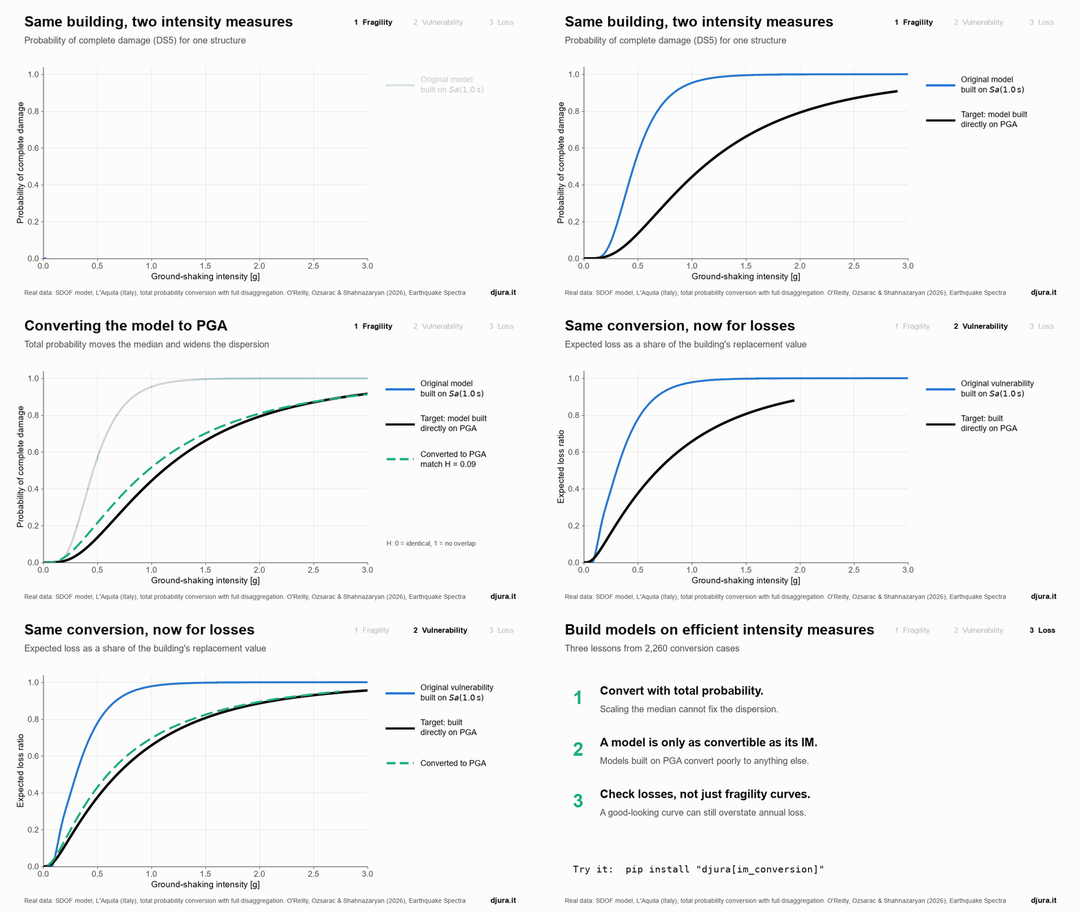
Why convert fragility and vulnerability models?

Fragility and vulnerability models are the backbone of any seismic risk analysis. A fragility function gives the probability that a structure exceeds a damage state (DS) for a given level of shaking, PDS > ds | IM = im. A vulnerability function gives the expected loss for that same level of shaking, EL | IM = im. Both are conditioned on an intensity measure (IM), the single number used to describe how strong the ground shaking is.

The trouble is that there is no single agreed IM. Some models use peak ground acceleration (PGA), others use spectral acceleration at a given period, Sa(T), and more recent studies use next-generation IMs such as average spectral acceleration, Sa_avg(T), or filtered incremental velocity, FIV3(T). Each choice is reasonable on its own. Put them together in a regional risk model, however, and you run into a problem.

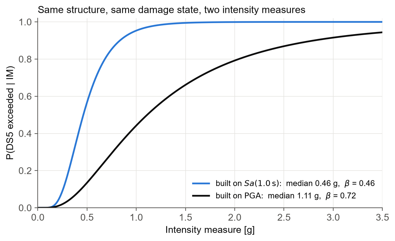
Imagine two research groups who publish fragility models for the same building class. One builds theirs on PGA, the other on Sa(1.0 s). The figure below shows exactly that situation for one of the structures examined here: same structure, same damage state, two IMs. The curves look completely different, and there is no way to tell by eye whether they agree, because their horizontal axes measure different things.

When a portfolio of buildings is analysed together, the ground motion fields must be simulated for every IM used in the models, and they must be correlated with one another. Those cross-correlated fields are expensive to generate, and the models needed to generate them are seldom available. A risk modeller then has three options:

1. 1. Use a single IM for every model and simulate one ground motion field.
2. 2. Keep each model's own IM and simulate several cross-correlated ground motion fields.
3. 3. Convert every model to a common IM, so that one ground motion field serves them all.

This post is about the third option: how to convert a fragility or vulnerability model from one IM to another, which methods work, and when conversion can be trusted. It summarises the study of O'Reilly, Ozsarac and Shahnazaryan (2026), and shows how to run the conversion yourself with the djura Python package (pip install "djura[im_conversion]").

How do you convert a model?

There are two broad families of approach. The first scales the model using the seismic hazard; the second integrates over everything the hazard says about the two IMs.

1. Scaling the median

The simplest idea is to keep the dispersion of the fragility function as it is and only move its median. The question is then how far to move it.

• Uniform hazard spectrum scaling (Silva et al. 2014) takes the scaling factor from a design spectrum. It only works between Sa(T) values.
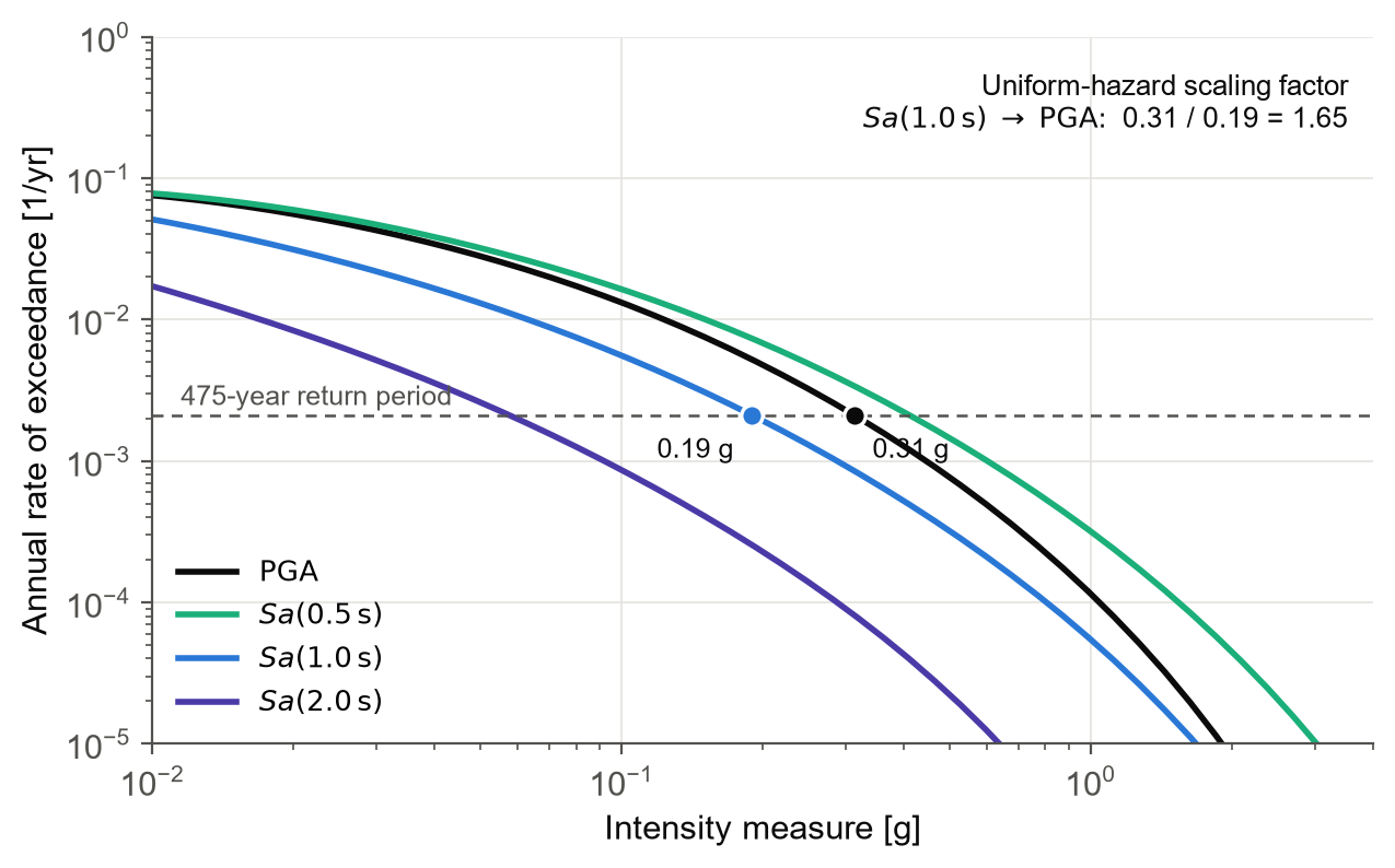
• Hazard curve scaling (O'Reilly and Calvi 2020) takes the scaling factor from the site hazard curves. Find the value of each IM with the same return period, and their ratio is the scaling factor. This also works for IMs that are not Sa(T).
• Uniform risk (trialled in O'Reilly et al. 2026) uses the fact that the annual rate of exceeding a damage state should be the same, whichever IM is used to compute it. Equating the two closed-form risk integrals gives the new median.

The figure below shows the hazard curve approach at L'Aquila, Italy, the site used throughout this post. At the 475-year return period, Sa(1.0 s) is 0.19 g and PGA is 0.31 g, so the scaling factor is 1.65. A fragility median of 0.46 g in Sa(1.0 s) would become 0.76 g in PGA.

These methods are quick and need very little information. They also rest on a strong assumption: that the two IMs explain the structural response equally well, so the dispersion does not need to change. As we will see shortly, that is rarely true.

2. Total probability

The more rigorous approach applies the total probability theorem (Suzuki and Iervolino 2020). For a given value of the target IM, im2, you ask: what values of the original IM are likely to go with it? You then average the original fragility over those values:

P[DS | IM2 = im2] = ∫ P[DS | IM1] · f(IM1 | IM2 = im2, Rup) · f(Rup | IM2 = im2) dIM1 dRup

Three ingredients go into this integral:

• PDS | IM1, the original fragility model that you already have.
• f(IM1 | IM2, Rup), how one IM predicts the other for a given earthquake scenario. This is the same conditional distribution that conditional spectrum record selection uses, built from a ground motion model and an IM correlation model.
• f(Rup | IM2), how much each earthquake scenario contributes to shaking at im2. This comes from the hazard disaggregation, and it is where the site enters the calculation.

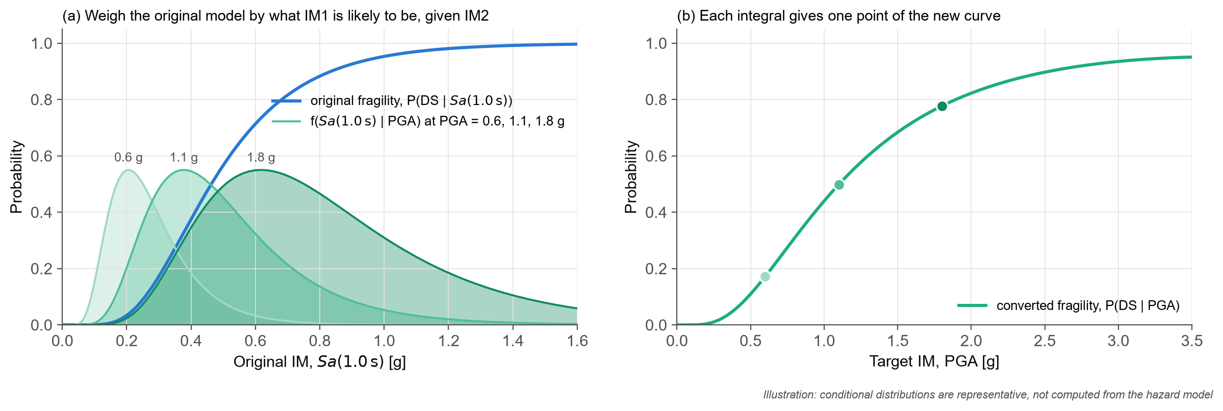
The figure below illustrates the idea. On the left, the blue curve is the original fragility in Sa(1.0 s). For each value of PGA, the green distribution shows the Sa(1.0 s) values that are likely to occur together with it. Multiply the two and integrate, and you get one point of the converted curve on the right. Repeat for every PGA value and you have the converted fragility. Note that the converted curve comes out with its own dispersion: nothing forces it to match the original one.

Two extensions were made in this work. First, the integral uses the complete disaggregation output of the OpenQuake engine (every rupture parameter and every ground motion model) rather than magnitude and distance alone. Second, the same integral is applied to vulnerability functions, simply by replacing the fragility with the expected loss:

E[L | IM2 = im2] = ∫ E[L | IM1] · f(IM1 | IM2 = im2, Rup) · f(Rup | IM2 = im2) dIM1 dRup

Vulnerability conversion had not been examined before, and it matters because many risk models are delivered as vulnerability, not fragility.

The seven methods compared

The full disaggregation is not always available, so three simplified versions were also tested. Together with the scaling methods, this gives seven methods, ordered here from most to least hazard information:

• Method 1: total probability with the full disaggregation.
• Method 2a: total probability with enough rupture scenarios to cover 50% of the hazard.
• Method 2b: total probability with the mean scenario of the disaggregation.
• Method 2c: total probability with the modal scenario of the disaggregation.
• Method 3: design spectrum scaling (Silva et al. 2014), Sa(T) only.
• Method 4: hazard curve scaling (O'Reilly and Calvi 2020).
• Method 5: uniform risk equivalence.

How do we know a conversion is right?

To score a conversion, we need to know the right answer. So every structure was analysed directly in every IM, giving a reference model built on the target IM. The converted model is then compared against it.

The study used four single-degree-of-freedom systems in OpenSees, with five damage states each. The site was L'Aquila, Italy, with the ZS9 source model and the Aristeidou et al. (2024) ground motion model. Ground motions were selected with the conditional spectrum method through the Djura record selector, 40 records per intensity level, and multiple stripe analysis gave fragility functions in 18 IMs. A damage-to-loss model then turned the fragility functions into vulnerability functions. In total, 2,260 conversion cases were tested.

The figure below shows the system used in all the examples of this post (model 2, T = 1.0 s), the damage-to-loss model, and how its five fragility functions combine into one vulnerability function.

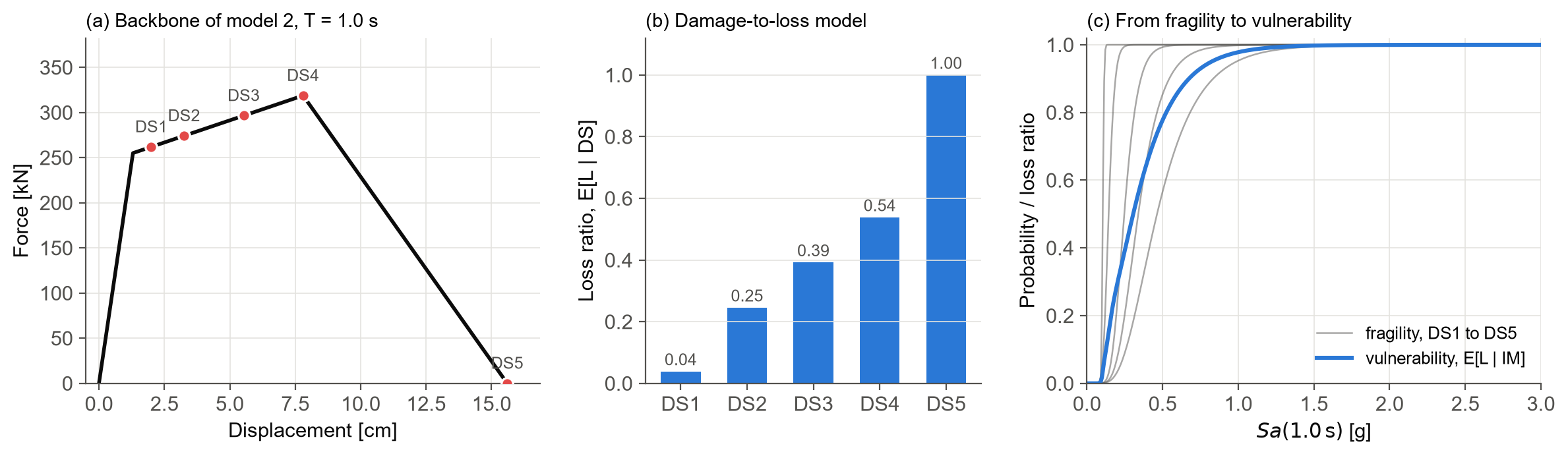
The match between a converted and a reference fragility is measured with the Hellinger distance, H. It compares two probability distributions with one number between 0 (identical) and 1 (nothing in common). That makes it possible to summarise thousands of cases in a single figure.

Results for fragility functions

Total probability works; the full disaggregation is optional

Let's return to the example from the start: a fragility model in Sa(1.0 s), converted to PGA. The figure below shows all seven methods against the reference model built directly on PGA.

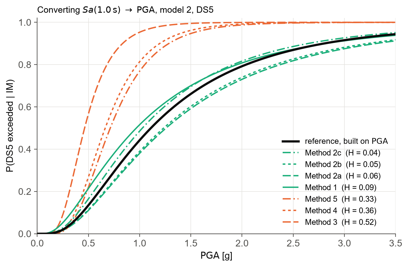
The total probability methods (green) all track the reference closely, with H between 0.04 and 0.09. The scaling methods (orange) sit far to the left, with H between 0.33 and 0.52. They keep the dispersion of the Sa(1.0 s) model, but PGA explains the response of this structure less well, so the true PGA fragility is much wider. The median is off too. The hazard curve scaling factor is 1.65, yet the ratio between the two reference medians is 2.4.

The more useful finding is within the green group. Going from the full disaggregation (Method 1) to a single mean or modal scenario (Methods 2b and 2c) costs almost nothing in accuracy. You need a probabilistic treatment, but you do not need every rupture scenario in your hazard model. This held across the whole study.

Efficiency decides what can be converted

Why do some conversions work and others fail? The answer lies in the IMs themselves, and you can see it before any conversion takes place.

The figure below shows four reference fragility functions for the same structure and damage state, each built on a different IM. The intensity is normalised by each curve's own median, so the only visible difference is the spread. PGA gives a dispersion of 0.72; Sa(1.0 s) gives 0.46; Sa_avg3(1.0 s) and FIV3(1.0 s) both give 0.17.

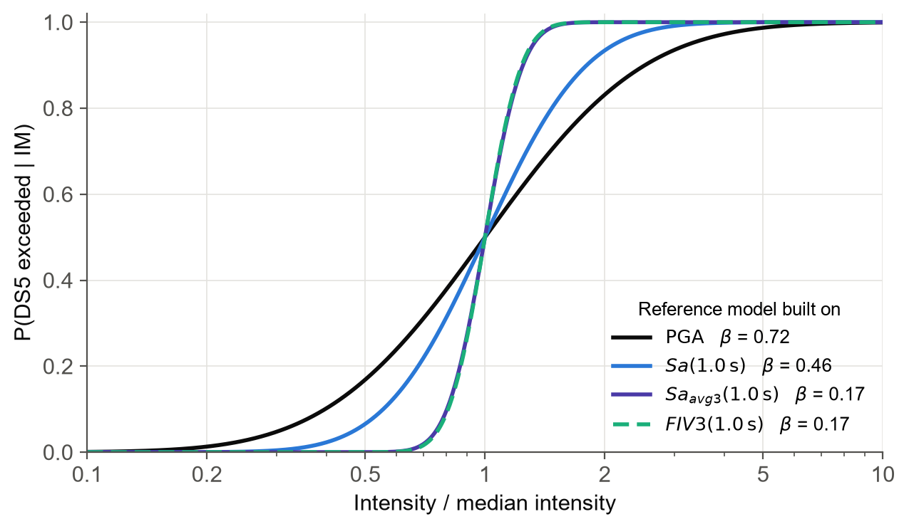
A steep curve means the IM explains the structure's response well: we call it efficient. A flat curve means much of the response is left unexplained. That unexplained spread is information the model has already lost, and no conversion can put it back. The integral only redistributes what the original model contains.

Direction matters

The same reasoning explains why a conversion can work in one direction and fail in the other. Converting from an efficient IM to a less efficient one works. Converting from an inefficient IM to an efficient one does not.

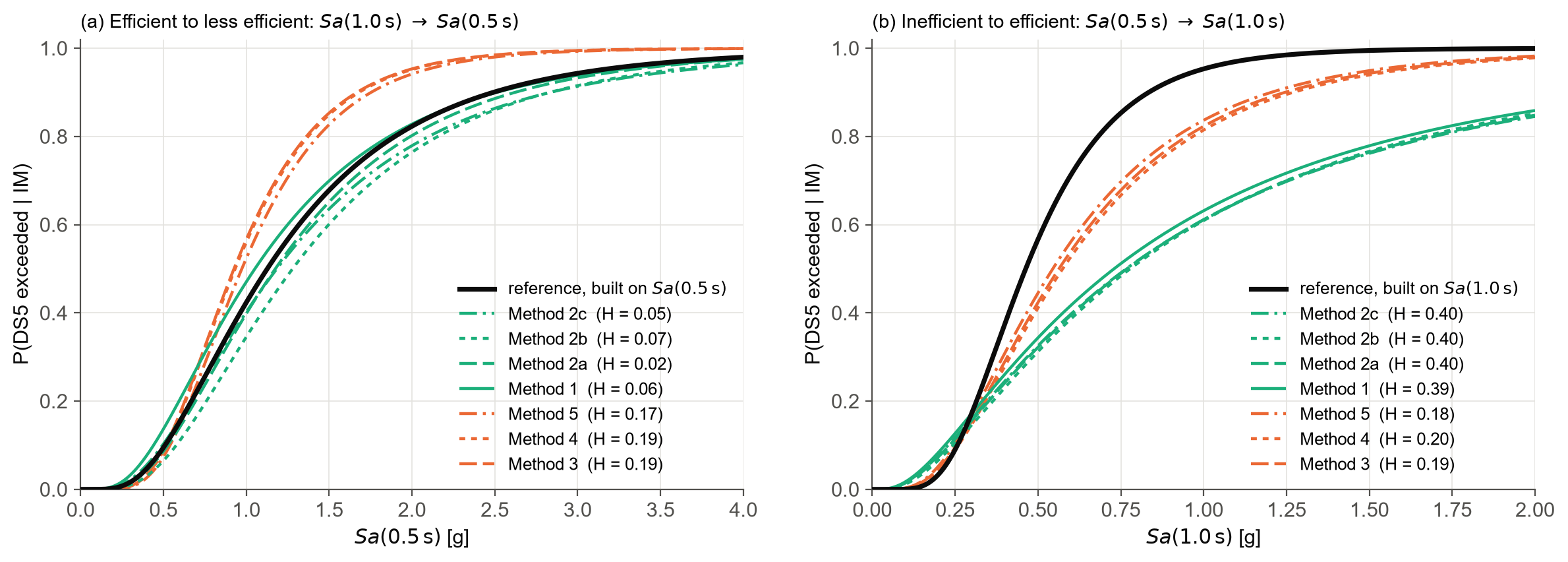
On the left, Sa(1.0 s) is converted to Sa(0.5 s). For this 1.0 s structure, Sa(1.0 s) is the more efficient IM (dispersion 0.46 against 0.62), and the total probability methods land on the reference (H = 0.02 to 0.07). On the right is the reverse, Sa(0.5 s) to Sa(1.0 s), and every method misses (H around 0.4 for total probability).

Why is Sa(0.5 s) such a poor starting point? It measures the shaking at a period well below the structure's own period of 1.0 s. As the structure is damaged and yields, it softens and its effective period lengthens, moving even further away from 0.5 s. A short-period IM therefore misses both the structure's period and its period elongation. That response information was never captured in the original model, so the conversion has nothing to recover it from: the conditional distribution in the integral becomes wide and poorly constrained. This is why, for Sa(T)-based IMs, conversions towards shorter periods tend to work and conversions towards longer periods tend to fail. The period itself is not the cause; efficiency is.

There is a trap worth pointing out in the right-hand panel. The scaling methods appear to do better here (H around 0.19). They are not better. Holding the dispersion fixed simply limits how far wrong they can go. It caps the visible error; it does not fix the conversion.

The whole picture: PGA receives, FIV3 donates

The heat map below summarises every pair of IMs for the mean scenario method (2b), averaged over the five damage states. The original IM is on the vertical axis and the target IM on the horizontal. Pale cells are good conversions; dark red cells are poor ones.

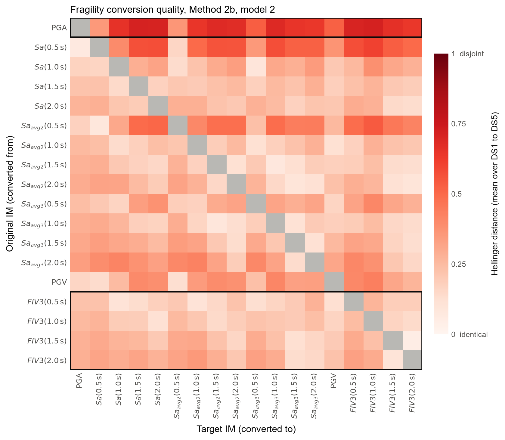
Two patterns stand out:

• The PGA row is dark red (mean H = 0.62). A model built on PGA cannot be converted to anything better: the information is already gone. Read down the PGA column, however, and most cells are pale (mean H = 0.24). Other IMs convert into PGA quite well.
• The FIV3 rows are pale throughout. A model built on FIV3(T) converts reasonably to every target, and FIV3 at different periods converts easily between its own definitions, because it is nearly period-independent.

Borrowing the terminology of blood transfusion: PGA is a universal receiver, and FIV3(T) is a universal donor. The short-period rows, Sa(0.5 s) and Sa_avg2(0.5 s), tell the same story as above. For this 1.0 s structure they are inefficient, so they only convert well towards PGA, which is even less efficient.

Results for vulnerability functions

Vulnerability converts more easily than fragility

Now the same integral, applied to vulnerability. The figure below shows two cases, with the four total probability methods against the reference.

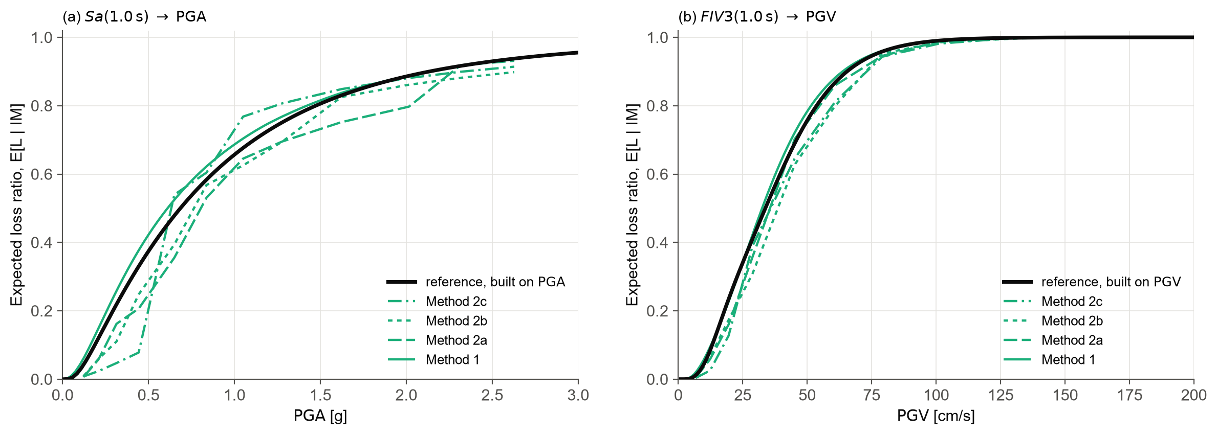
At the loss level, the choice of method matters much less. The full disaggregation and the simplified scenarios land close to each other and to the reference, and the match is best at low intensities, which is where most of the annual loss accumulates. The simplified methods are a little jagged in the left-hand panel because they are evaluated at fewer intensity levels; their overall trend is still right.

But converting to PGA overestimates losses

Since everything converts into PGA, harmonising a whole portfolio on PGA might look like a sensible engineering decision. The fragility curves match, after all.

To check what that does to risk, each converted vulnerability function was integrated with the site hazard to get the average annual loss (AAL), and compared with the AAL of the reference model.

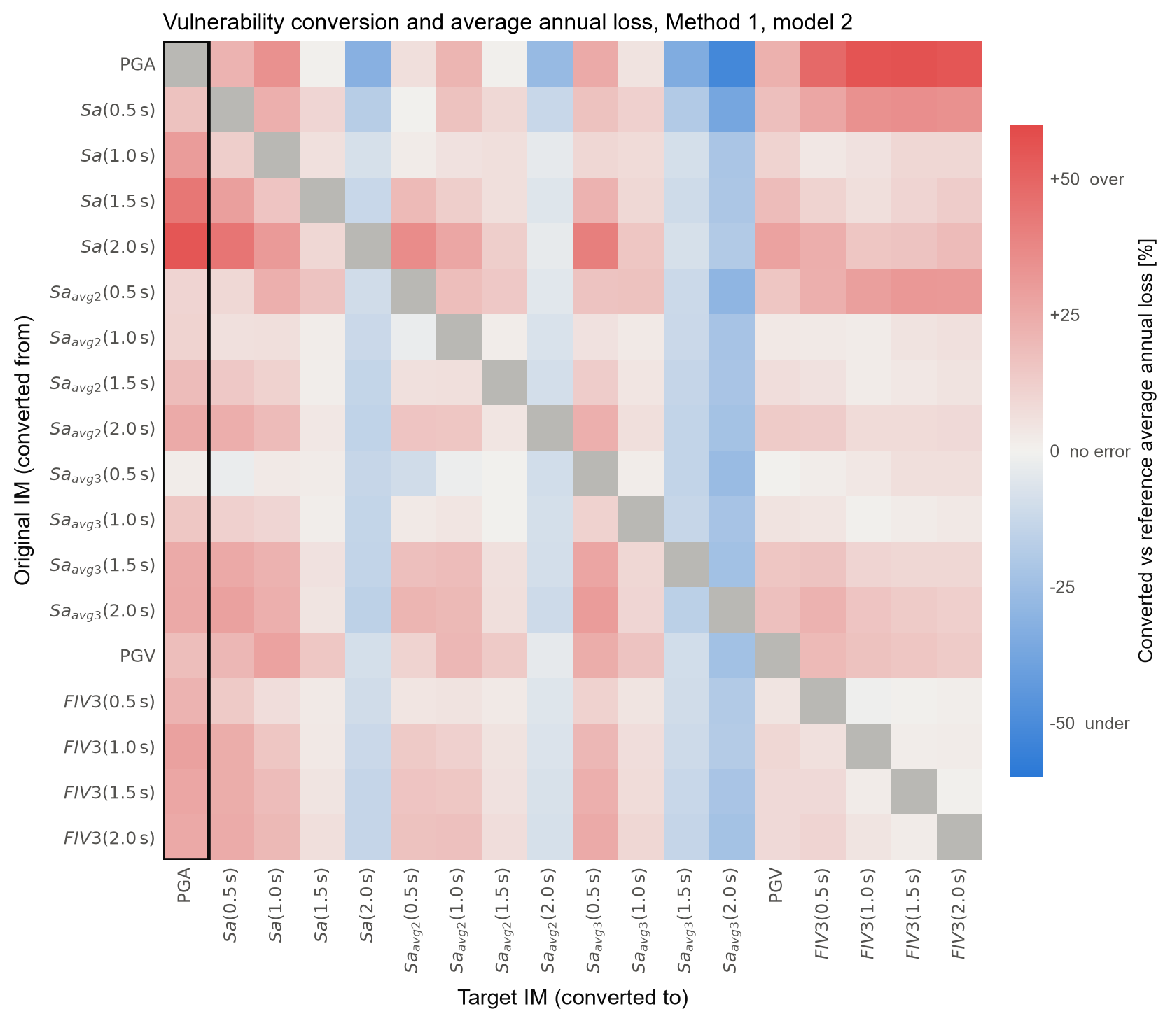
The PGA column, the very column that looked acceptable at the fragility level, is red in every row. Converting to PGA overestimates the AAL in every case: by +30% for our Sa(1.0 s) example, by +23% on average and by up to +55%. For comparison, the same Sa(1.0 s) model converted to FIV3(1.0 s) is within 5%, and models built on FIV3(T) stay within about 10% on average for targets other than PGA. These values use Method 1. The simplified methods' vulnerability curves were stored on a coarse grid that starts at 0.12 g, which misses the low intensities where most of the annual loss accrues, so they are not used for AAL here. The reason PGA overestimates is dispersion again. A PGA-based model is wide; a wide model raises the expected loss at every level of shaking; integrated over the hazard, that error builds up.

So a conversion can be visually correct at the fragility level and materially wrong at the loss level. If you only check the fragility, you will not see it.

Doing it yourself with djura

Both conversion approaches are available in the djura Python package, in the im_conversion module. Install it with:

pip install "djura[im_conversion]"

Total probability with the full disaggregation

FF takes an original fragility (median and dispersion in IM1), the target IM2 with the grid of values to evaluate, a ground motion model input file, and the OpenQuake disaggregation context for the site. The example below uses the input files shipped with the package tests: input.json and ctx.pickle.

import json
import pickle
from djura.im_conversion import FF

with open("input.json", encoding="utf-8") as f:
    base_input = json.load(f)          # GMM ensemble, site and rupture data
with open("ctx.pickle", "rb") as f:
    oq_data = pickle.load(f)           # OpenQuake disaggregation context

# Original fragility, defined in Sa(1.0 s)
im1 = {"median": 0.376, "dispersion": 0.295, "name": "SA(1.0)"}

# Target IM, evaluated from 0.001 to 5.0 g
im2 = {"name": "SA(0.5)", "min": 0.001, "max": 5.0, "num_pts": 100}

probs, im2_range = FF(im1, im2, data=base_input, dis_oq=oq_data).create()

probs is the converted fragility curve, evaluated at im2_range.

Converting a vulnerability function

To convert a vulnerability function, pass the original curve as discrete points instead of a median and dispersion. im_range holds the IM1 values and probs holds the expected loss ratios:

im1 = {
    "name": "SA(1.0)",
    "im_range": vulnerability_ims,     # IM1 values
    "probs": vulnerability_losses,     # E[L | IM1] at those values
}
losses, im2_range = FF(im1, im2, data=base_input, dis_oq=oq_data).create()

Checking the result

To score a conversion against a reference model, fit a lognormal distribution to the converted curve and compute the Hellinger distance. Note that hellinger_distance expects the logarithm of the median:

import numpy as np
from djura.record_selection.utilities import fit_cdf_to_data
from djura.record_selection.metrics import hellinger_distance

fit = fit_cdf_to_data(im2_range, probs, distribution="lognormal",
                      method="least_squares")

# Reference fragility built directly on Sa(0.5 s)
ref_median, ref_dispersion = 0.733, 0.354

h, _ = hellinger_distance(np.log(ref_median), ref_dispersion,
                          fit["mu"], fit["sigma"])
print(f"median {np.exp(fit['mu']):.2f} g, beta {fit['sigma']:.2f}, H {h:.2f}")

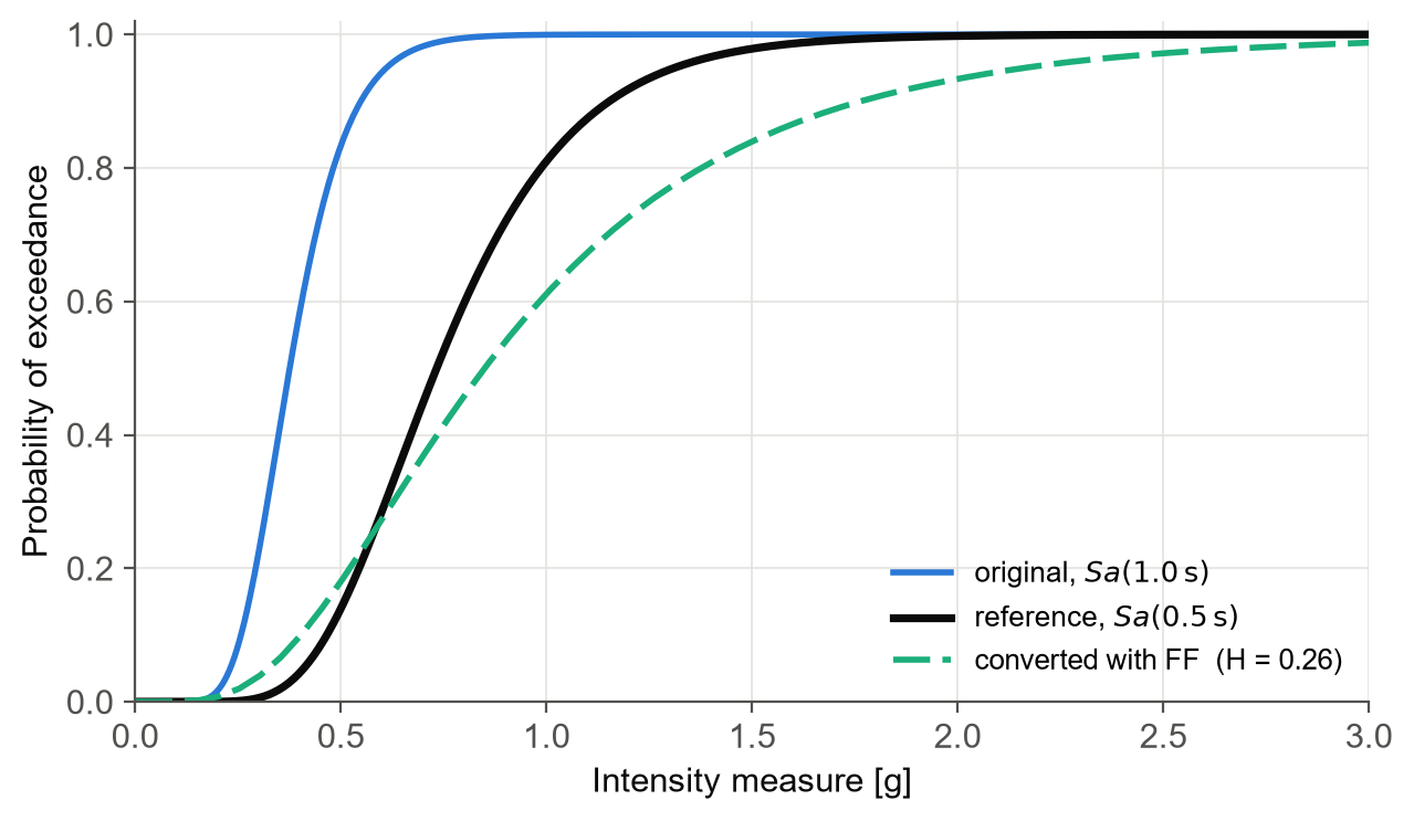
For this example the converted fragility has a median of 0.85 g and a dispersion of 0.57, against a reference of 0.73 g and 0.35, giving H = 0.26. The figure below shows the result.

Without a full disaggregation

If you do not have a disaggregation context, FFApproximate runs the same total probability conversion from a pre-computed input file that holds the representative scenarios for the site, as in Methods 2a to 2c. The example input files are approx_SA(0.5).json and ff.json.

from djura.im_conversion import FFApproximate

with open("approx_SA(0.5).json", encoding="utf-8") as f:
    approx_input = json.load(f)

im1 = {"median": 0.376, "dispersion": 0.295, "name": "SA(1.0)"}
im2 = {"name": "SA(0.5)"}

probs, im2_range = FFApproximate(im1, im2, data=approx_input).create()

Given the results above, this is usually all you need.

Conclusion

Summary

This post looked at how to convert seismic fragility and vulnerability models from one intensity measure to another, so that models from different sources can be compared and run on a single ground motion field.

First, total probability methods consistently outperform the simpler scaling methods, because they let the dispersion change along with the median. A mean or modal disaggregation scenario gives almost the same accuracy as the full disaggregation.

Second, efficiency decides what can be converted. A model is only as convertible as the IM it was built on. Converting from an efficient IM to a less efficient one works; converting from an inefficient IM to an efficient one does not, because the information the original IM never captured cannot be recovered. PGA is a universal receiver: other IMs convert into it, but models built on it cannot be converted out. FIV3(T) is a universal donor: models built on it convert well to any target.

Third, vulnerability converts more easily than fragility, and the method matters less at the loss level. However, harmonising models on PGA overestimates the average annual loss, by 23% on average and up to 55% in this study, even when the fragility curves appear to match.

The practical advice is simple. For as long as we work with fragility and vulnerability models, build new ones on efficient, next-generation IMs such as Sa_avg(T) or FIV3(T). They convert in any direction, and they can be reused by people who did not build them. And if losses are your end product, convert the vulnerability model directly.

Limitations and future work

All results here come from a single site. Hazard enters the conversion equations directly, so whether these findings hold in other tectonic settings is still an open question, and the next one to answer. Kohrangi et al. (2017) suggest that next-generation IMs such as Sa_avg(T) may be less site-dependent than Sa(T), which would make them even more attractive.

Conversion is also not the only route. Where several IMs can be simulated together through cross-IM spatial correlation models (Monteiro et al. 2026), conversion may not be needed at all. Conversion is for the many models that already exist and will not be rebuilt.

All plots for every case in the study, along with the computational tools, are available in the GitHub repository.

Stay Tuned

Get in touch if you would like to use this service by visiting the website or dropping us an email. Stay tuned for more posts, and contact us for more information.

References

• O'Reilly GJ, Ozsarac V, Shahnazaryan D (2026) Conversion of Seismic Fragility and Vulnerability Models to Alternative Intensity Measures for Regional Risk Analysis. Earthquake Spectra 42: e70098. DOI: 10.1002/esp4.70098
• Suzuki A, Iervolino I (2020) Intensity measure conversion of fragility curves. Earthquake Engineering & Structural Dynamics 49(6): 607–629. DOI: 10.1002/eqe.3256
• Silva V, Crowley H, Colombi M (2014) Fragility Function Manager Tool. In: SYNER-G: Typology Definition and Fragility Functions for Physical Elements at Seismic Risk. Springer. DOI: 10.1007/978-94-007-7872-6_13
• O'Reilly GJ, Calvi GM (2020) Quantifying seismic risk in structures via simplified demand–intensity models. Bulletin of Earthquake Engineering 18(5): 2003–2022. DOI: 10.1007/s10518-019-00776-0
• Cornell CA, Jalayer F, Hamburger RO, Foutch DA (2002) Probabilistic Basis for 2000 SAC Federal Emergency Management Agency Steel Moment Frame Guidelines. Journal of Structural Engineering 128(4): 526–533. DOI: 10.1061/(ASCE)0733-9445(2002)128:4(526)
• Aristeidou S, Shahnazaryan D, O'Reilly GJ (2024) Artificial neural network-based ground motion model for next-generation seismic intensity measures. Soil Dynamics and Earthquake Engineering 184: 108851. DOI: 10.1016/j.soildyn.2024.108851
• Aristeidou S, Shahnazaryan D, O'Reilly GJ (2025) Correlation models for next-generation amplitude and cumulative intensity measures using artificial neural networks. Earthquake Spectra 41(1): 851–875. DOI: 10.1177/87552930241270563
• Dávalos H, Miranda E (2019) Filtered incremental velocity: A novel approach in intensity measures for seismic collapse estimation. Earthquake Engineering & Structural Dynamics 48(12): 1384–1405. DOI: 10.1002/eqe.3205
• Kohrangi M, Vamvatsikos D, Bazzurro P (2017) Site dependence and record selection schemes for building fragility and regional loss assessment. Earthquake Engineering & Structural Dynamics 46(10): 1625–1643. DOI: 10.1002/eqe.2873
• Monteiro VA, Aristeidou S, O'Reilly GJ (2026) Spatial Cross-Correlation Models for Next-Generation Amplitude and Cumulative Intensity Measures. Earthquake Spectra 42(2). DOI: 10.1002/esp4.70076
• Pagani M, Monelli D, Weatherill G, et al. (2014) OpenQuake Engine: An Open Hazard (and Risk) Software for the Global Earthquake Model. Seismological Research Letters 85(3): 692–702. DOI: 10.1785/0220130087
• Hellinger E (1909) Neue Begründung der Theorie quadratischer Formen von unendlichvielen Veränderlichen. Journal für die reine und angewandte Mathematik 136: 210–271. DOI: 10.1515/crll.1909.136.210