Generalised Unconditional Ground Motion Record Selection for Rupture Scenario(s)
The record selector used in this post is described in Shahnazaryan, Ozsarac and O'Reilly (2025), COMPDYN 2025, doi:10.7712/120125.12444.25126.
Introduction
Selecting ground motion records for nonlinear time-history analysis is critical for accurate seismic design and assessment. There are several methods available—ranging from simple building code requirements to more complex hazard scenarios and mainshock-aftershock sequences. In this post, we’ll explore one particular approach: selecting records using a set of target spectra for various ground motion intensity measures (IMs) based on specific rupture parameters, which is also known as scenario-based analysis, or generalised unconditional selection.
For a deeper dive into other selection methods, such as those conditioned on a particular intensity measure or related to mainshock-aftershock sequences, check out our other videos on YouTube and follow us on LinkedIn for more updates.
The table below compares scenario-based selection with the two other approaches in Djura's record selector: code-based selection to a uniform hazard spectrum and conditional spectrum selection for multiple stripe analysis.
| Method | Target | Hazard input | Intensity measures | Typical use |
|---|---|---|---|---|
| UHS / code-based | Code response spectrum, matched over a period range of interest | Building code parameters, or uniform hazard spectra retrieved from site coordinates (EFEHR, USGS, Türkiye) | Spectral acceleration | Code-compliant analysis to Eurocode 8, ASCE 7-22, NTC 2018, TBEC 2018 or SIA |
| Unconditional (scenario-based) | Distributions of IMs predicted by GMMs for one or more rupture scenarios | Rupture parameters and site context | PGA, SA(T), PGV, significant duration, Saavg, FIV3 | Shaking expected for a given rupture scenario |
| Conditional (CS / GCIM) | Distributions of IMs conditional on a known value of one conditioning IM | Conditioning value from the hazard curve or PSHA; rupture scenarios from disaggregation | PGA, SA(T), PGV, significant duration, Saavg, FIV3 | Hazard-consistent records for multiple stripe analysis |
Let’s dive into Djura’s Record Selector!
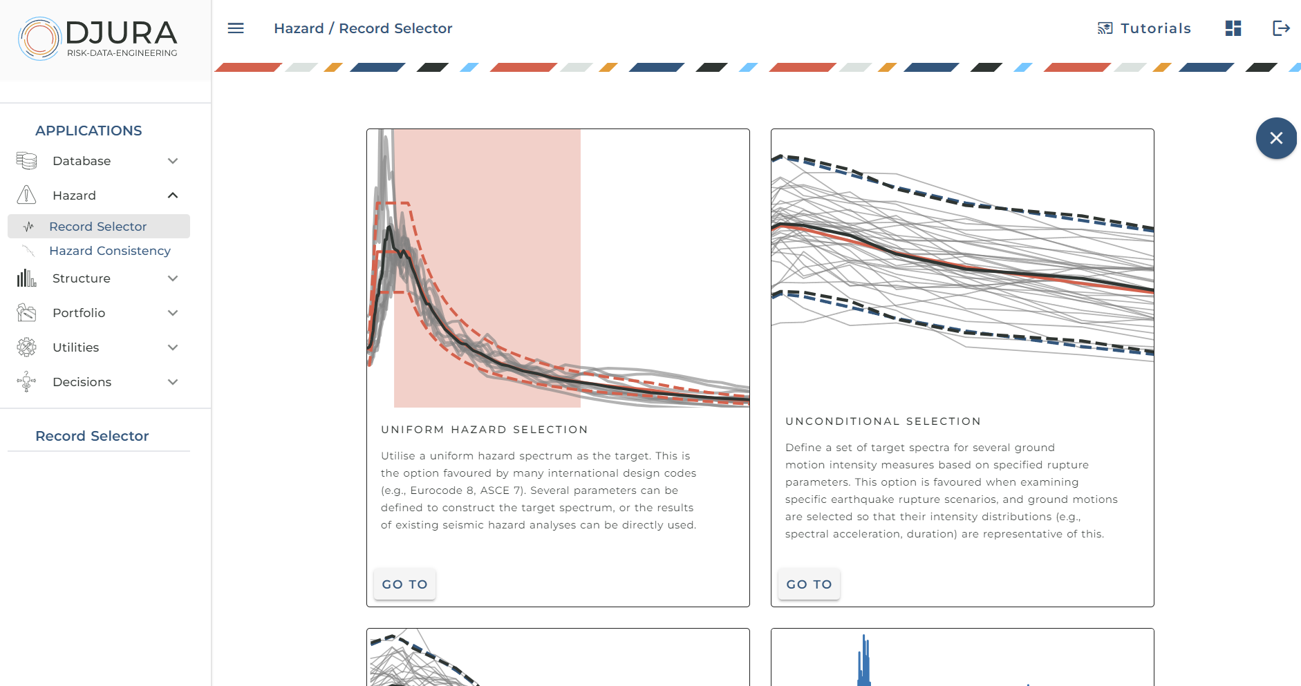
Add IM - GMMs pairs
An unconditional spectrum (UCS) is the expected probabilistic distribution of seismic intensity measures (IMs) for a given set of earthquake rupture parameters, without conditioning on the value of any one IM. To predict these distributions, we rely on ground motion models (GMMs). The first step is to identify which IMs we are interested in, which will determine the necessary GMMs.
To begin, click on “Add IM-GMM Pairs”.
How to Add an IM-GMM Pair
Let’s first define the IMs we’re focusing on and which GMMs we want to use to predict their expected distribution.
After clicking the “Add IM-GMM Pairs” button, you’ll see a list of available IMs, such as peak ground acceleration, PGA, spectral acceleration, SA(T), and significant duration, among others. This tool also includes options for more advanced next-generation IMs like average spectral acceleration (e.g., Vamvatsikos & Cornell, 2005; Eads et al., 2015; among others) and FIV3 (Dávalos & Miranda, 2019), which is a unique feature of this tool.
Let’s select SA as our first IM.
Choosing GMMs for an IM
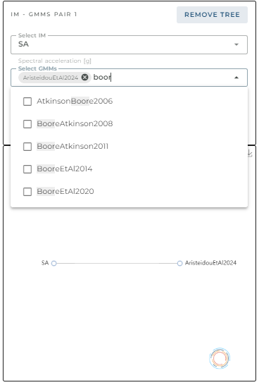
Once you’ve selected an IM like SA, a menu will appear showing the available GMMs. You can select one or more GMMs to predict the distribution of this IM and assign weights to each model. This feature of allowing multiple GMMs to be used to establish the target distribution is a unique feature of the Djura Record Selector as it allows analysts to account for different GMMs and more accurately represent what is carried out in seismic hazard analyses studies.
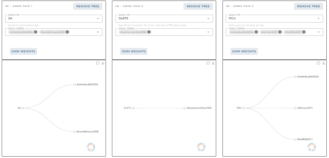
For example, let’s choose the AristeidouEtAl2024 and BooreAtkinson2008 GMMs. As you make these selections, the graphic below populates with your chosen GMMs and their respective weights, which default to being equal. You can adjust the weights by clicking “GMM Weights”, but for now, let’s leave them as is.
Adding non-SA IMs
One of the great and distinguishing features of this tool is the ability to include multiple IMs beyond just spectral acceleration (SA). By accounting for multiple IMs and their correlations, you can ensure that the ground motions selected represent not only SA but also other parameters like velocity and duration. While the theoretical details behind this approach are beyond the scope of this guide, you can find more information in Tarbali & Bradley (2015), for example.
Let’s add another IM, such as significant duration. Click “Add IM-GMM Pairs” again and choose significant duration 5-75, which is defined between 5% and 75% of Arias intensity. You’ll notice the available GMMs are different for this IM. This time, we’ll select only the AbrahamsonSilva1996 GMM.
Now, let’s add PGV (Peak Ground Velocity) as another IM. After clicking to add another pair, select PGV, and you’ll see new GMM options appear. For this example, let’s choose AristeidouEtAl2024, Atkinson2015, and BindiEtAl2011.
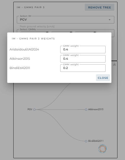
You can also adjust the weights for these GMMs. For instance, let’s assign weights of 0.4, 0.4, and 0.2, respectively. The tool automatically normalizes the values if they don’t add up to 1.
Downloading and Uploading IM-GMM Data
Once you’ve set up your IM-GMM pairs, you can download the data by clicking “Download Data”. This feature allows you to save the configuration, and you can later upload the same file to continue working on it or modify it programmatically. Simply use the Upload button on the right-hand side to reload your IM-GMM pairs.
[
  {
    "ID": 0,
    "SA": {
      "names": [
        "AristeidouEtAl2024",
        "BooreAtkinson2008"
      ],
      "weights": [
        0.5,
        0.5
      ]
    }
  },
  {
    // other IM-GMM pairs
  }
]
Now that we’ve defined the IMs and GMMs we’re interested in, it’s time to move forward. Click on Scenarios to continue to the next step.
Defining Rupture Scenarios
After defining the IM-GMM pairs in the previous step, the required parameters for the rupture scenarios will vary depending on the selected models. Each GMM may have slightly different input requirements, so the fields you need to fill out will appear based on the specific GMMs you've chosen.
Let’s walk through the main Scenario page to see how this works.
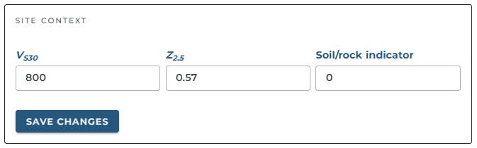
Defining the Site Context
The first step is to define the site context, which refers to the properties of the site itself rather than the earthquake rupture. Even though these parameters aren’t directly related to the earthquake, they are still required by the GMMs to accurately estimate ground motion.
- : The average shear-wave velocity in the upper 30 meters of the site.
- and Soil/Rock Indicator: These parameters may vary between GMMs, and while we won’t dive into their details here, you can hover over the fields for brief descriptions. Full explanations can be found in the respective GMM's documentation.
Some default values are provided to help you get started, but you should replace these with values specific to your study.
Defining the Rupture Parameters
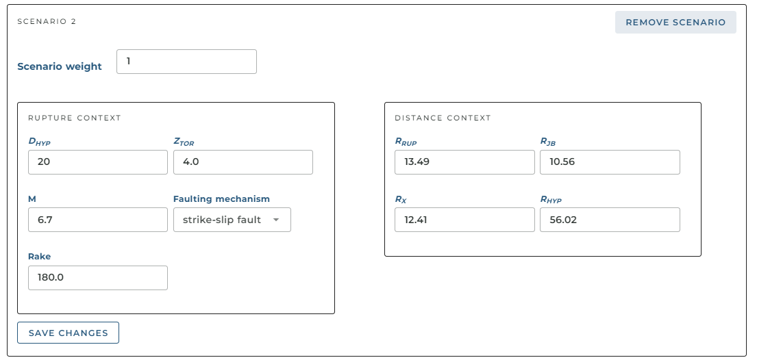
Next, we move on to defining the rupture parameters for each scenario. To do this, click “Add”, and a new box will appear with the necessary fields.
For each rupture scenario, the selected GMMs will estimate the IM distributions. As with the site context, default values are pre-filled to guide you, but it’s important to update them based on your study.
A powerful feature of the Djura Record Selector is the ability to add multiple rupture scenarios and assign relative weights to them. This feature is unique, allowing for more comprehensive analysis by accounting for different potential rupture events in your study area.
For this example, let’s add a second scenario with slightly different values—such as modifying the magnitude—to demonstrate how the tool manages multiple scenarios.
Downloading and Uploading Rupture Scenario Data
Just like with the IM-GMM pairs, you can download the rupture scenario data as a JSON file. This is particularly useful because the data is presented in a dictionary format, making it easy to modify and process programmatically, especially for batch processing tasks.
You can also upload previously saved JSON files to quickly reload your scenario data, streamlining your workflow.
Visualise Logic Tree
Once you’ve set up your scenarios and are satisfied with your input, you can visualise the logic tree. This takes you to a separate page where all the details about IMs, GMMs, weights, rupture scenarios, and other parameters are listed in a table format.
The table allows you to search for specific IMs, GMMs, or rupture parameters to check exact details such as their associated weights and selected GMMs. This is especially useful for double-checking or fine-tuning the inputs you've defined.
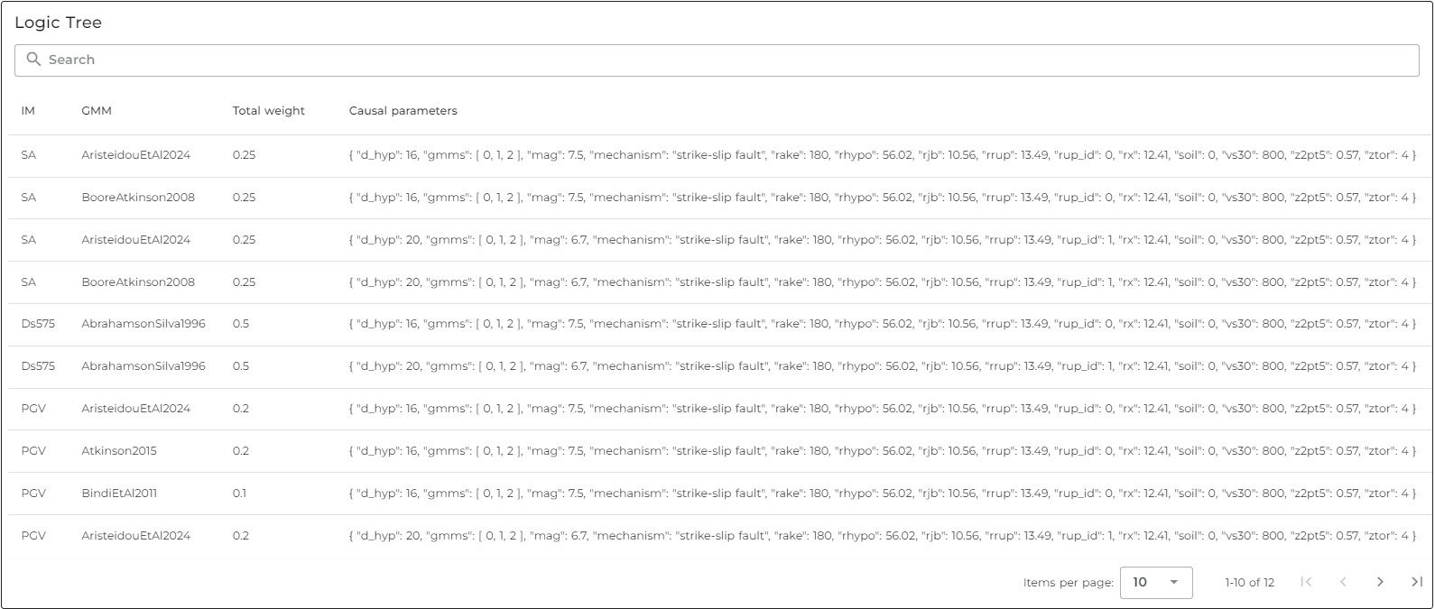
For a more intuitive representation, the tool also provides an interactive logic tree diagram. This diagram offers a clear, global view of what is being analyzed, making it easier to understand the relationships between rupture scenarios, IMs, and GMMs.
The diagram starts with the rupture scenarios—in this case, we had two scenarios. For each rupture, the diagram shows:
- The IMs being predicted.
- The GMMs used to estimate their distributions.
You can hover over each element in the diagram to see the specific weights assigned to each IM and GMM. The diagram is interactive, meaning you can collapse or expand sections to view as much or as little detail as needed.
This visual representation can be saved for use in publications or reports, adding a professional touch to your analysis. Additionally, the full table used to generate the diagram can be downloaded for further review or modification.
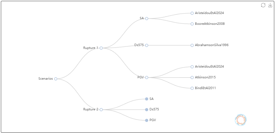
The logic tree provides a comprehensive overview of your selection process, combining both a detailed table and an interactive diagram. This dual-visualisation approach helps ensure that your inputs are correctly defined and makes it easy to present your findings in a clear and organized manner.
Advanced Input
Before creating the target distribution, there are several advanced input parameters that can be defined and tailored depending on your preferences.
Advanced Selection and Computational Settings
One of the first options involves the number of horizontal components and the type of horizontal definition to be used. You can choose between options such as:
- Geomean: Geometric mean of the two components.
- RotD100: Maximum rotated component.
- RotD50: Median rotated component.
Additionally, you will specify the number of required ground motions and set scaling limits. The Kolmogorov-Smirnov test significance level is also set here, which is used for statistical testing, and is typically left at 5%.
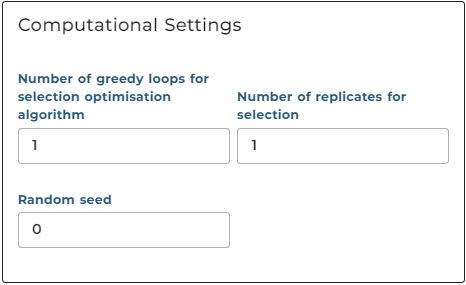
The computational settings section on the right-hand side relates to the number of loops required to obtain a good match between the ground motion records and the target spectrum.
In most cases, the default values for these settings will work well, so unless specific adjustments are needed, they can be left as is.
Intensity Measures (IMs)
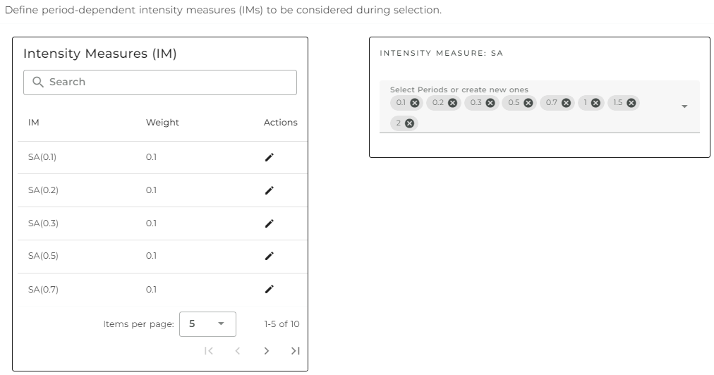
One important aspect that hasn’t been discussed in depth yet is the definition of intensity measures (IMs), particularly spectral acceleration (SA). Since SA is a period-dependent IM, we need to specify the periods of vibration at which it is measured.
By default, several periods are pre-selected. If you need to add a specific period (e.g., SA(1.2s)), you can simply type 1.2 and hit enter. This will automatically add the period to the list of period-dependent IMs, and the selection criteria and weights will update accordingly.
Causal Earthquake Rupture Parameter Limits
The final advanced input parameter relates to any causal earthquake parameter limits you may want to place on the ground motions selected.
For example, you may want to limit the ground motions to those within a specific magnitude range or select motions from a particular faulting style. Additional information, such as site-specific parameters or rupture characteristics, can also be specified here. However, these limits are optional and can be left out if they are not required for your analysis.
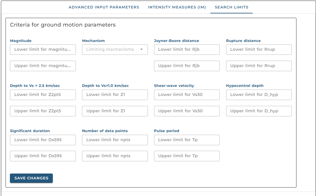
These advanced input parameters offer more control over the ground motion selection process, ensuring that the records selected match your analysis needs as closely as possible. Once you’ve adjusted the parameters to your satisfaction, you can proceed with generating the target distribution and performing the record selection.
Create Target IM Distribution
Validating the Downloading the Input Data
Before generating the target distribution, it’s important to validate your input. This ensures that everything has been set up correctly, and all required parameters are in place.
To validate, simply click the "Validate" button on the right-hand side. This quick check helps confirm that your input is ready for the next step.
You can also download all the input data you’ve entered so far by clicking the "Download All Data" button. This saves your configurations, making it easier to review or share later.
Creating the Target IM Distribution
Once your input is validated, it’s time to create the target distribution. Click the "Create Target Distribution" button on the right-hand side. After doing so, a new menu called "Target Visualisation" will appear on the left-hand side, where you can view the results.
Understanding the Figures
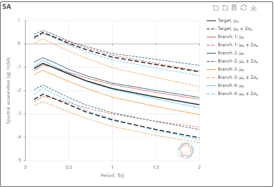
The Target Visualisation page displays the probabilistic distributions for each IM based on the selected GMMs and rupture scenarios. Unlike traditional methods that only consider a single rupture scenario or GMM, this tool allows you to account for multiple scenarios and models.
For period-dependent IMs, the tool presents the target median spectrum and percentiles based on the GMMs and rupture scenarios you’ve specified.
Take a moment to browse the figures and explore the target distributions for each IM.
For spectral acceleration (SA), you’ll notice there are 4 branches in the distribution. This is consistent with the logic tree setup—since we’ve defined two rupture scenarios and selected two GMMs, the 4 branches represent each combination of rupture and GMM.
Although the values are shown in logarithmic form, the dispersions (variability) are not. Below the figure, you’ll see that for SA, when multiple rupture scenarios and GMMs are used, they are combined to give the overall mean and standard deviation of the target distribution.
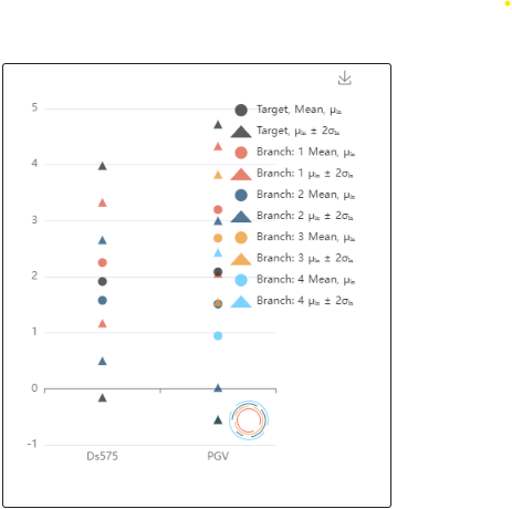
For non-period-dependent IMs like duration and PGV (Peak Ground Velocity), the visualisation shows the mean and dispersions for each branch of the logic tree. This provides a clear view of how these parameters vary across different rupture scenarios and GMMs.
Browse these figures to gain insights into the expected values for these non-period-dependent IMs.
Saving the Figures
The figures in the Target Visualisation section are fully interactive, allowing you to toggle different layers on and off. This makes it easier to focus on specific branches or data points as needed.
You can also save the figures for use in presentations, reports, or further analysis. This feature is especially useful for documenting your work and sharing results with others.
The ability to interact with, analyze, and save the target distribution figures adds a layer of flexibility and depth to your ground motion selection process. Once you’ve explored the results, you can move forward with the selection and analysis, knowing that your input is validated and your target IM distribution is well-defined.
Perform the Selection
Once all your inputs are validated and your target IM distribution is ready, it’s time to perform the record selection. This process is extremely fast and runs in a split second. After the selection is complete, a new menu called “Selection Visualisation” will appear on the left-hand side.
To start the selection, click the "Perform Record Selection" button on the right-hand side.
Interpreting Period-Dependent Figures
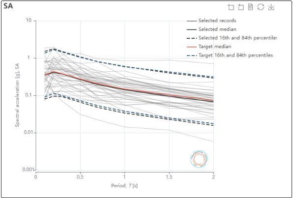
In the Selection Visualisation section, you’ll find figures similar to the ones seen earlier, but now they represent the selected ground motions compared to the overall target.
Each individual ground motion selected is displayed alongside the mean and standard deviations of the target distribution. You’ll be able to clearly see that the target and selected spectral acceleration (SA) values match closely, indicating a successful selection process.
The plot is interactive, allowing you to:
- Turn off specific layers for better inspection.
- Zoom in and out for a closer look at certain data points.
- View the tabular data behind the figures.
- Save the figure for use in presentations or reports.
Take some time to browse the period-dependent figures and explore how well the selection fits your target distribution.
Exploring Cumulative Distributions for Each IM
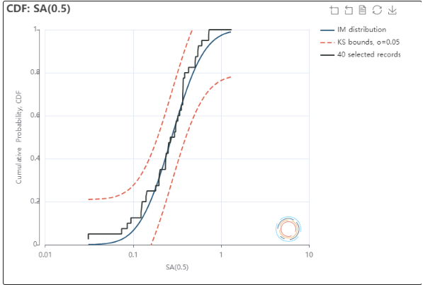
From the dropdown menu, you can also explore the cumulative distribution functions (CDFs) for each IM. These figures show how well the selected records match the target distribution.
For each IM, you’ll see the cumulative distribution for the selected ground motions compared to the target, as well as the KS (Kolmogorov-Smirnov) limits, which help evaluate the quality of the match.
Use the dropdown menu to select different target IMs and inspect their corresponding CDFs.
Viewing and Downloading the Earthquake Data
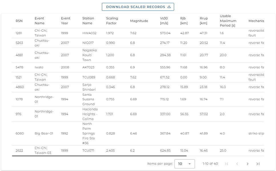
Below the figures, you’ll find a table containing the metadata for the selected ground motion records. This table allows you to quickly verify that all the necessary requirements have been met for your analysis.
Browse through the metadata to confirm that the ground motions selected align with your project needs.
Downloading the Selected Records
Once you’re satisfied with the selection, you can download the ground motion records. Simply click the “Download Scaled Records” button to get a ZIP file that contains all the selected data.
The ZIP file includes all the information you need to begin your analysis, providing a convenient way to store and share the data.
By following these steps, you’ve successfully selected ground motions that match your target IM distribution. The interactive figures and downloadable data make it easy to evaluate, present, and share your results. Now you can move forward with confidence, knowing that your selection is optimized for your seismic analysis.
Conclusion
Summary
In this post, we explored a simple and efficient method for ground motion record selection based on unconditional spectra for specific intensity measures (IMs), selected ground motion models (GMMs), and rupture scenarios. This approach is particularly useful for identifying the shaking intensity for a given rupture scenario, ensuring that the distribution of IMs for the selected ground motions is representative and consistent with the scenario being analyzed.
Future Updates
We are continuously enhancing the tool’s capabilities and adding features based on user feedback. Upcoming improvements include:
- Expanding our ground motion databases to give users access to even more data.
- Enhancing interoperability with other services to provide a more integrated experience.
The accompanying video tutorial provides a step-by-step guide on using the UI, making record selection a breeze.
In the near future, the tool will also be callable via API for Python or MATLAB, allowing seamless integration into your workflow with a single command.
Further reading
- Conditional spectrum record selection for multiple stripe analysis: selecting records conditioned on a known value of one intensity measure.
- Code-based ground motion record selection using uniform hazard spectra: selecting and scaling records to a building code spectrum.
- Ground motion signal processing in Python: computing intensity measures such as Saavg and FIV3 from a record.
Stay Tuned
This is just one of the many ground motion selection tools we offer. Visit our website or contact us to learn more, or see our risk engineering consulting services.
Stay tuned for more updates, videos, and tools to help streamline your seismic analysis.
Frequently asked questions
What is scenario-based ground motion record selection?
Scenario-based, or unconditional, record selection picks ground motions whose intensity measures match the distributions predicted by ground motion models for one or more specified earthquake rupture scenarios. It is useful for identifying the shaking intensity expected for a given rupture scenario.
What is the difference between unconditional and conditional record selection?
Unconditional selection targets the IM distributions predicted for a set of rupture parameters. Conditional selection also fixes a known value of one conditioning IM, typically from probabilistic seismic hazard analysis, and builds the target for the other IMs around it.
Can I use more than one ground motion model in record selection?
Yes. In the Djura record selector each IM can be predicted by several GMMs with user-defined weights, which are normalised automatically if they do not add up to 1. Combined with multiple rupture scenarios, this gives a logic tree with one branch per rupture and GMM.
Which intensity measures can be used in scenario-based selection?
PGA, SA(T), PGV, significant duration, average spectral acceleration and FIV3, among others. Accounting for several IMs and their correlations makes the selected records representative of velocity and duration as well as spectral acceleration.
References
- Shahnazaryan, D., Ozsarac, V., & O’Reilly, G. J. (2025) "Djura ground motion record selector: a software solution for earthquake engineering" COMPDYN 2025. DOI: 10.7712/120125.12444.25126
- Dávalos, H., & Miranda, E. (2019). Filtered incremental velocity: A novel approach in intensity measures for seismic collapse estimation. Earthquake Engineering & Structural Dynamics, 48(12), 1384–1405. https://doi.org/10.1002/eqe.3205
- Vamvatsikos, D., & Cornell, C. A. (2005). Developing efficient scalar and vector intensity measures for IDA capacity estimation by incorporating elastic spectral shape information. Earthquake Engineering & Structural Dynamics, 34(13), 1573–1600. https://doi.org/10.1002/eqe.496
- Eads, L., Miranda, E., & Lignos, D. G. (2015). Average spectral acceleration as an intensity measure for collapse risk assessment. Earthquake Engineering & Structural Dynamics, 44(12), 2057–2073. https://doi.org/10.1002/eqe.2575
- Aristeidou, S., Shahnazaryan, D., & O’Reilly, G. J. (2024). Artificial neural network-based ground motion model for next-generation seismic intensity measures. Soil Dynamics and Earthquake Engineering, 184, 108851. https://doi.org/10.1016/j.soildyn.2024.108851
- Boore, D. M., & Atkinson, G. M. (2008). Ground-Motion Prediction Equations for the Average Horizontal Component of PGA, PGV, and 5%-Damped PSA at Spectral Periods between 0.01 s and 10.0 s. Earthquake Spectra, 24(1), 99–138. https://doi.org/10.1193/1.2830434
- Tarbali, K., & Bradley, B. A. (2015). Ground motion selection for scenario ruptures using the generalised conditional intensity measure (GCIM) method. Earthquake Engineering & Structural Dynamics, 44(10), 1601–1621. https://doi.org/10.1002/eqe.2546
- Gail M. Atkinson; Ground‐Motion Prediction Equation for Small‐to‐Moderate Events at Short Hypocentral Distances, with Application to Induced‐Seismicity Hazards. Bulletin of the Seismological Society of America 2015;; 105 (2A): 981–992. doi: https://doi.org/10.1785/0120140142
- Bindi, D., Pacor, F., Luzi, L. et al. Ground motion prediction equations derived from the Italian strong motion database. Bull Earthquake Eng 9, 1899–1920 (2011). https://doi.org/10.1007/s10518-011-9313-z
- Vamvatsikos, D., & Cornell, C. A. (2005). Developing efficient scalar and vector intensity measures for IDA capacity estimation by incorporating elastic spectral shape information. Earthquake Engineering & Structural Dynamics, 34(13), 1573–1600. https://doi.org/10.1002/eqe.496
- Abrahamson, N. A., and Silva, W. J., 1996. Empirical Ground Motion Models, Report to Brookhaven National Laboratory.