Ground Motion Signal Processing - Intensity Measures, Spectra and Pulses in Python

From a recorded ground motion to the numbers engineers use
Every seismic assessment starts from ground motion records. A record on its own is just a long list of accelerations sampled every few milliseconds. To select records, scale them, build fragility models or compare a record against a hazard target, we need to turn that list into a handful of meaningful numbers: how strong the shaking was, how long it lasted, which frequencies it carried, and how a structure would respond to it. Those numbers are the intensity measures (IMs): an intensity measure is a single number that summarises one aspect of a ground motion record, such as its strength, duration or frequency content.
Computing them looks simple, but the details matter. Which definition of spectral acceleration do you use? How do you combine the two horizontal components? How fine must the time step be for the response spectrum to be right? Does the record contain a near-fault velocity pulse?
The signal_processing module of the djura Python package (pip install "djura[signal_processing]") answers all of these in one place. It reads records, computes more than thirty intensity measures, rotates horizontal pairs to any RotDxx definition, conditions records with baseline correction and filtering, and identifies velocity pulses. This post walks through each of these using a single real record, so you can see what every measure means and how to get it in a line of Python.
The record we will use
Throughout this post we use NGA-West2 RSN 179: the 1979 Imperial Valley earthquake recorded at El Centro Array #4. It is a well-known near-fault record, which makes it a good test case for pulse identification later on. Both horizontal components ship with the package tests, so you can reproduce everything below.
Reading a record
read_nga reads PEER NGA files (.AT2) and returns the time step, the number of points, the header description, the time vector and the acceleration in g. Records from the European ESM database are read with read_esm, and convert_esm_to_peer_format writes them out in PEER format.
import numpy as np
from djura import signal_processing as sig

dt, npts, desc, t, acc1 = sig.read_nga("RSN179_IMPVALL.H_H-E04140.AT2")
_, _, _, _, acc2 = sig.read_nga("RSN179_IMPVALL.H_H-E04230.AT2")

h1 = sig.Component(acc1, dt, unit="g")
print(h1)
# <Component npts=7818 dt=0.005 duration=39.09 s PGA=0.4843 g solver=exact>
A Component holds one acceleration trace. If your record is not in g, pass its unit ("m/s2", "cm/s2" or "gal") and it is converted on the way in. From here on, scalar measures are properties and spectral measures are methods that take the periods. Every value is cached, so asking twice costs nothing.
Acceleration, velocity and displacement
The first thing to look at is the record itself. The velocity and displacement histories are obtained by integrating the acceleration, and their peaks give the three classic measures: peak ground acceleration (PGA), peak ground velocity (PGV) and peak ground displacement (PGD).
h1.pga, h1.pgv, h1.pgd      # 0.48 g, 39.6 cm/s, 25.1 cm
vel, disp = h1.vel, h1.disp # the full histories, in cm/s and cm
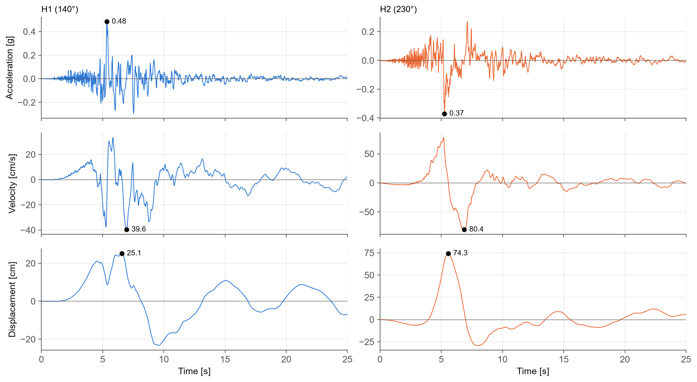
The two components tell different stories. H1 (140°) has the larger acceleration peak, 0.48 g, but H2 (230°) has twice the velocity and three times the displacement. The single large, long velocity swing in H2 around 5 to 7 s is the signature of a near-fault pulse; we will come back to it at the end.
How strong, and for how long?
Peaks capture only one instant. Several measures summarise the whole record instead.
- Arias intensity (Ia) is proportional to the integral of the squared acceleration, and measures the total energy content of the shaking (Arias 1970). Here it is 1.36 m/s.
- Cumulative absolute velocity (CAV) is the integral of the absolute acceleration, 0.85 g·s.
- Root mean square values of acceleration, velocity and displacement (
arms,vrms,drms) give the average level of shaking, and the characteristic intensity (ic) combines RMS acceleration with duration.
Duration has several definitions, and the module provides all the common ones:
- Significant duration is the time between two fractions of the Arias intensity: 5 to 75% (D5-75) and 5 to 95% (D5-95) by default (Trifunac and Brady 1975), or any pair you choose.
- Bracketed duration is the time between the first and last time the acceleration exceeds a threshold.
- Uniform duration is the total time spent above that threshold.
h1.ia, h1.cav                        # 1.36 m/s, 0.85 g.s
h1.arms, h1.vrms, h1.drms, h1.ic
h1.ds575, h1.ds595                   # 2.7 s, 6.7 s
h1.significant_duration(0.05, 0.95)  # (start, end, duration) = (4.8, 11.5, 6.7) s
h1.bracketed_duration(0.05)          # 11.2 s
h1.uniform_duration(0.05)            # 4.1 s
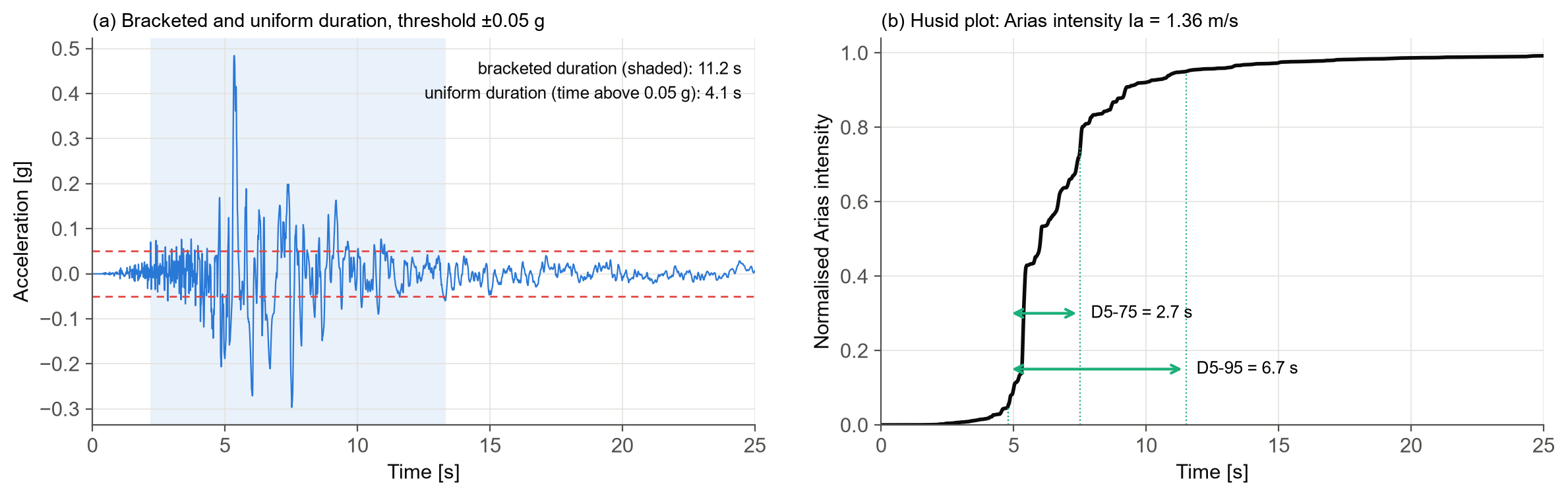
The right-hand panel is the Husid plot: the Arias intensity accumulated over time, normalised by its total. Most of the energy of this record arrives in a short burst after 5 s, which is why D5-75 is under 3 s even though the record lasts 39 s.
Frequency content
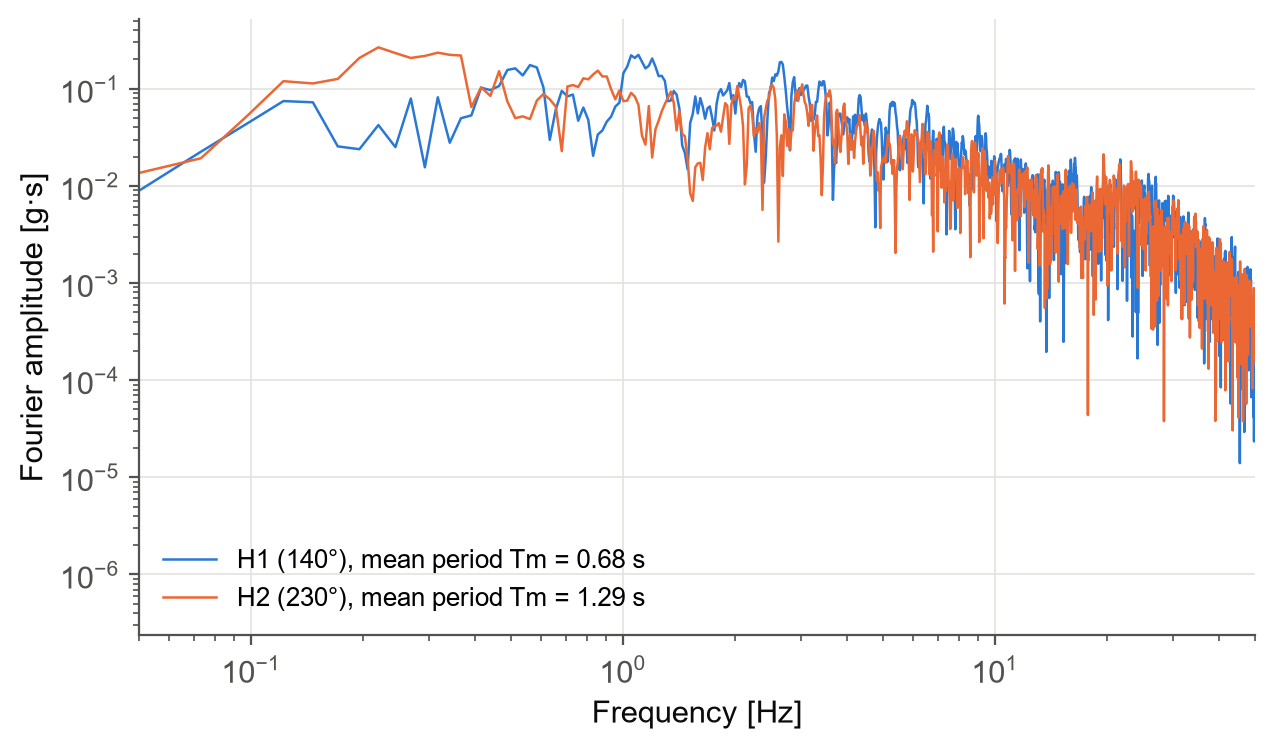
The Fourier amplitude spectrum (FAS) shows how the energy of the record is distributed over frequency. The power amplitude spectrum (PAS) is also available, and the mean period, Tm (Rathje et al. 1998), condenses the frequency content into a single number.
freq, amp = h1.fas    # Hz, g.s
freq, power = h1.pas
h1.tm                 # 0.68 s
Response spectra
Structures do not respond to the ground motion directly; they respond to it through their own dynamics. A response spectrum records the peak response of a series of single-degree-of-freedom (SDOF) oscillators, each with a different period, to the record. It is the most widely used tool in earthquake engineering.
The module computes the full family of spectra, with 5% damping by default:
- Relative displacement, Sd, the peak deformation of the oscillator.
- Pseudo-velocity, PSV = ω·Sd, and pseudo-acceleration, PSA = ω²·Sd. PSA is what design codes, ground motion models and record selection use when they say "spectral acceleration", Sa(T).
- The true velocity and acceleration spectra (
sv_rel,sa_abs) are computed directly from the relative and absolute response histories. - The predominant period, Tp, where the acceleration spectrum peaks.
periods = np.geomspace(0.02, 6.0, 140)

h1.psa(periods)      # g; h1.sa(periods) is an alias
h1.psv(periods)      # cm/s
h1.sd(periods)       # cm
h1.sa_abs(periods)   # true absolute acceleration, g
h1.sv_rel(periods)   # true relative velocity, cm/s
h1.tp(periods)       # 0.19 s
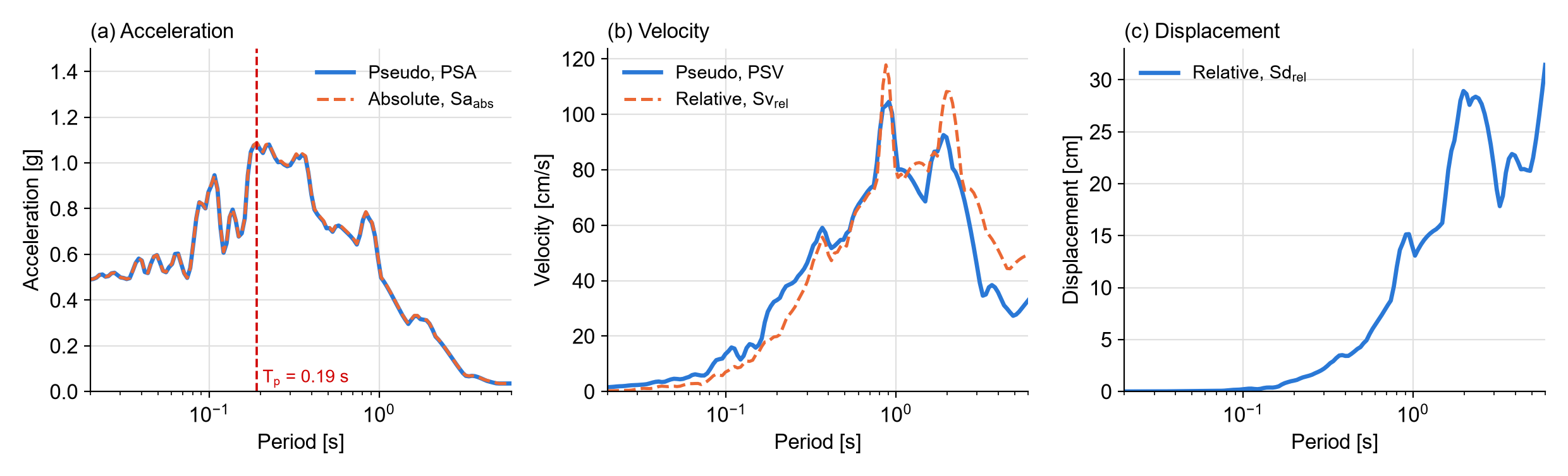
For an undamped oscillator, PSA and the true absolute acceleration are identical. With 5% damping they stay very close, within about 1% up to 1 s for this record, and the gap grows slowly with period (2.5% at 5 s). The velocity spectra differ much more. At short periods the pseudo-velocity exceeds the true relative velocity, while at long periods it underestimates it, and the gap generally widens as the period increases.
Spectrum intensities
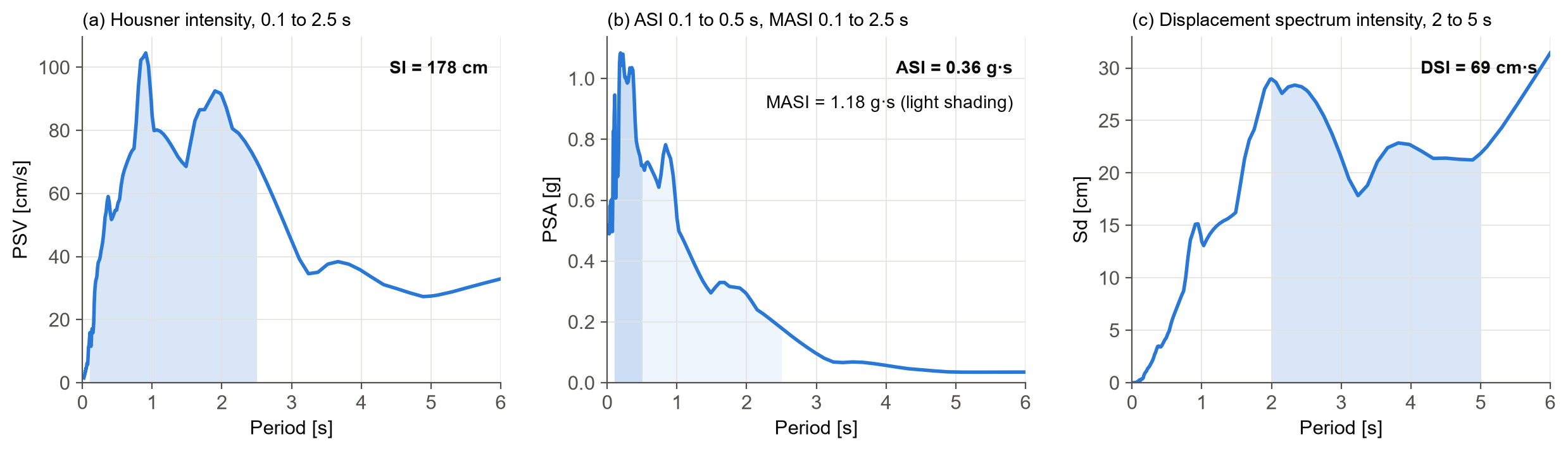
Integrating a spectrum over a band of periods gives a measure that is less sensitive to the exact period of a structure:
- Housner intensity (SI), the area under the PSV between 0.1 and 2.5 s (Housner 1952).
- Acceleration spectrum intensity (ASI), the area under the PSA between 0.1 and 0.5 s (Von Thun et al. 1988), suited to stiff structures such as dams.
- Modified acceleration spectrum intensity (MASI), the same area from 0.1 to 2.5 s.
- Displacement spectrum intensity (DSI), the area under Sd between 2 and 5 s (Bradley 2011), suited to flexible structures and geotechnical problems.
The integration limits can be changed. One practical point: the period grid must reach both ends of the band, so add the limits to your periods explicitly. If they are missing, the method returns NaN rather than extrapolating.
bands = np.unique(np.r_[periods, 0.1, 0.5, 2.0, 2.5, 5.0])

h1.si(bands)     # 178 cm
h1.asi(bands)    # 0.36 g.s
h1.masi(bands)   # 1.18 g.s
h1.dsi(bands)    # 69 cm.s
Input energy
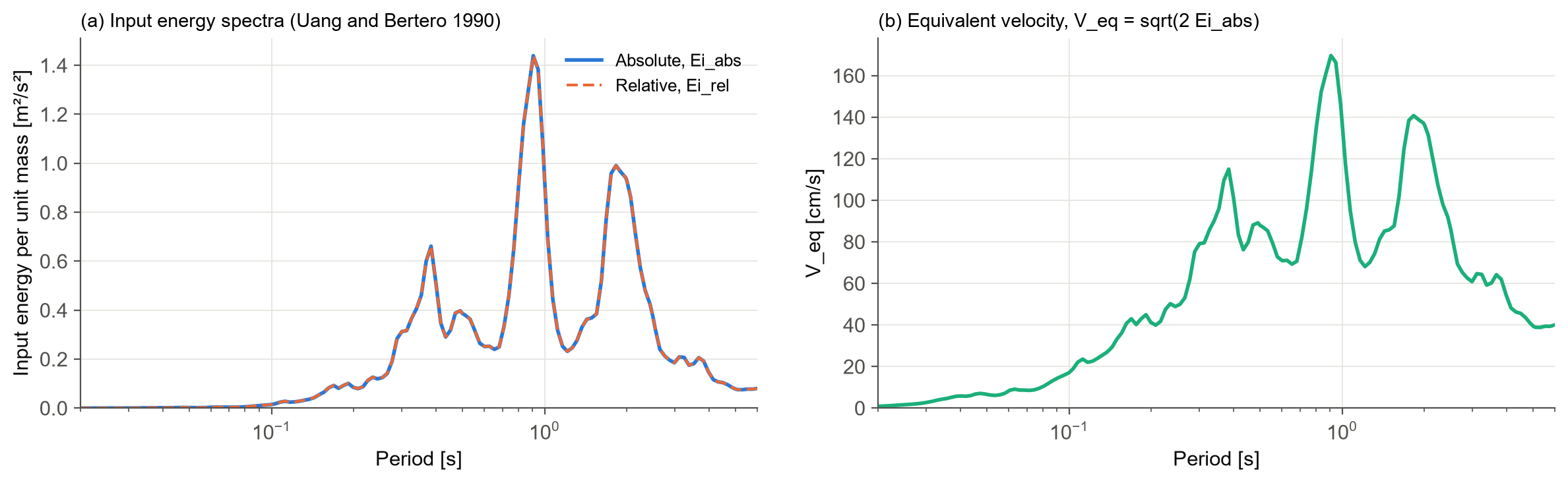
Peak response says nothing about how much energy the earthquake pushes into a structure, which governs cumulative damage. The input energy spectra of Uang and Bertero (1990) give that energy per unit mass, in its relative (ei_rel) and absolute (ei_abs) forms. The equivalent velocity, Veq = √(2 Ei,abs), expresses the same energy as a velocity.
h1.ei_rel(periods)   # m2/s2
h1.ei_abs(periods)   # m2/s2; 0.93 at 1.0 s
h1.v_eq(periods)     # cm/s; 136 at 1.0 s
Next-generation intensity measures
Sa(T) at a single period is the workhorse of practice, but it describes the shaking at only one period. A structure that yields softens, its period lengthens, and higher modes come into play, so the shaking at other periods matters too. Two next-generation IMs capture this and have been shown to predict structural response much better.
Average spectral acceleration
Average spectral acceleration, Saavg(T), is the geometric mean of Sa over a range of periods around T (Baker and Cornell 2006). By default the module averages 10 periods from 0.2T to 2.0T, and both bounds and the number of periods can be changed.
h1.sa_avg([1.0])                           # 0.50 g, over 0.2T to 2.0T
h1.sa_avg([1.0], t_low=0.2, t_high=3.0)    # 0.34 g, over 0.2T to 3.0T
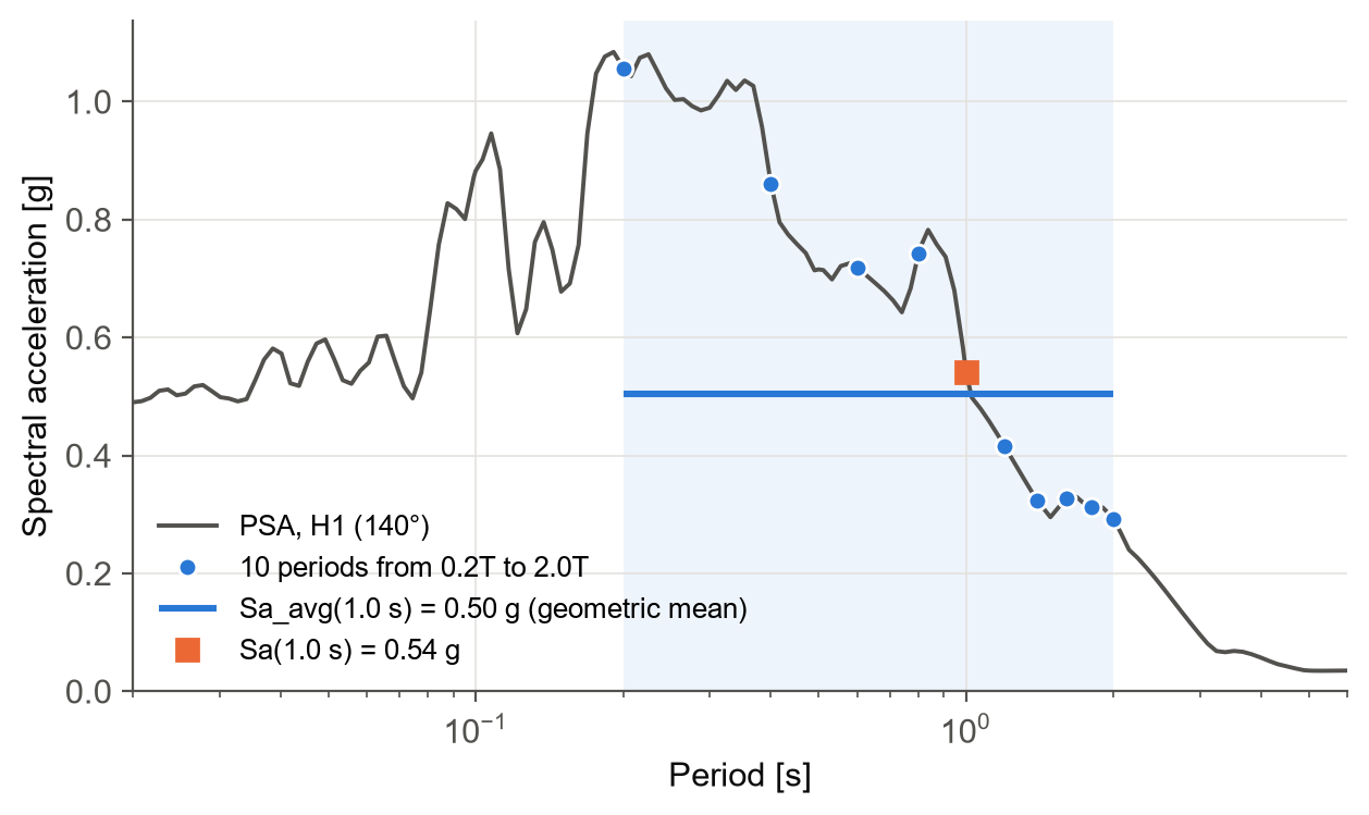
For this record, Sa(1.0 s) is 0.54 g and Saavg(1.0 s) is 0.50 g. The difference can be much larger for records whose spectra are jagged around T, which is exactly the information that Sa(T) alone misses.
Filtered incremental velocity
Filtered incremental velocity, FIV3(T) (Dávalos and Miranda 2019), works directly on the acceleration trace rather than on a spectrum. The record is first low-pass filtered to remove the high frequencies that do little damage to a structure of period T. The filtered acceleration is then integrated over sliding windows of 0.7T, which gives the velocity increment the ground delivers within each window. FIV3 is the larger of the sum of the three largest peaks and the sum of the three largest troughs.
h1.fiv3([1.0]) # 110 cm/s
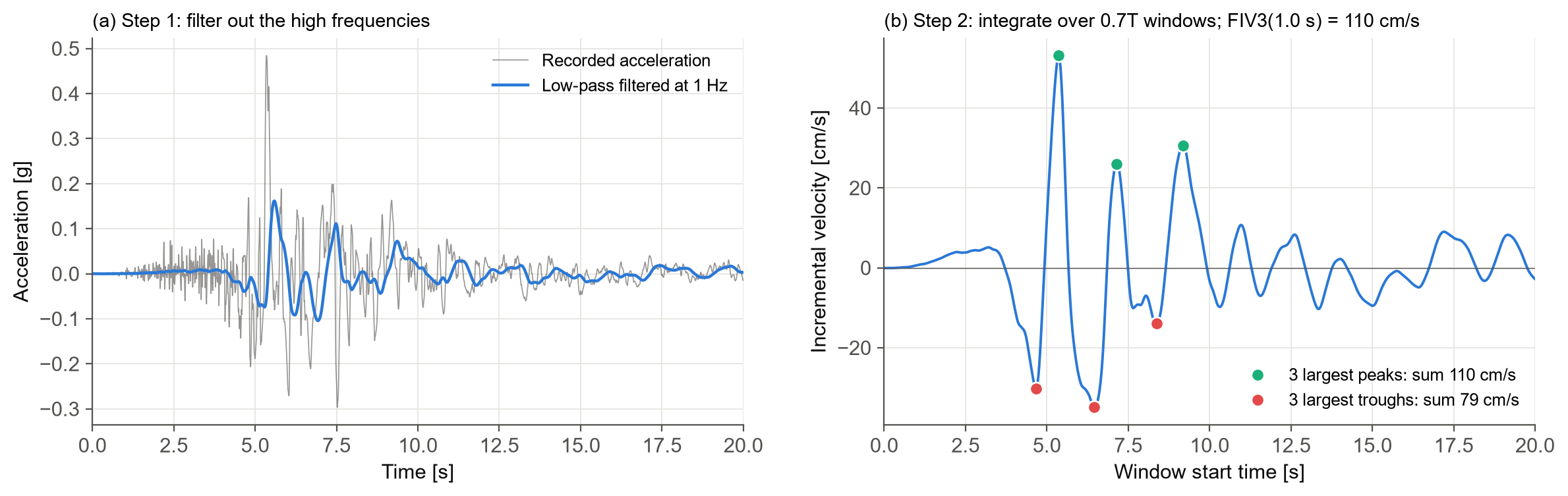
FIV3 responds to the large, coherent velocity increments that push a structure towards collapse, which is why it performs so well for collapse prediction. Its window length, filter cut-off and causal or acausal filtering can all be set (alpha, beta, filtering).
Two horizontal components: RotDxx
A record has two horizontal components, oriented however the instrument happened to be installed. Their individual spectra depend on that orientation, which has nothing to do with the earthquake. Modern ground motion models therefore use orientation-independent definitions (Boore 2010): rotate the pair through every angle from 0° to 180°, compute the measure in each direction, and take a percentile across angles. RotD50 is the median over all angles, and RotD100 is the maximum.
A GroundMotion holds the two horizontal components (and optionally the vertical), and its rotd method gives any percentile of any measure:
pair = sig.GroundMotion(acc1, acc2, dt)
pair.precompute(periods, sa_avg_periods=[1.0])   # solve the rotated SDOFs once

sa50, sa100 = pair.rotd("psa", [50, 100], periods)
pair.rotd("pga", [50, 100])          # RotD50 and RotD100 of PGA
pair.rotd("ia", 50)                  # any scalar measure
pair.rotd("sa_avg", 50, [1.0])       # Sa_avg in each direction, then the median
pair.rotd("fiv3", 50, [1.0])

pair.geomean("psa", periods)         # geometric mean of the two components
pair.at_angle("psa", 0.0, periods)   # one direction; 0 and 90 are the as-recorded ones
pair.first.pga, pair.second.pgv      # each component is a full Component
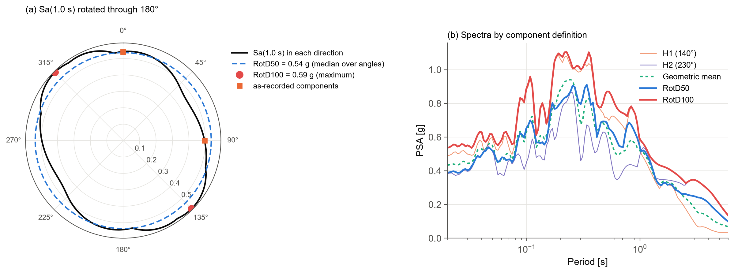
The left panel shows Sa(1.0 s) in every direction. RotD50 is 0.54 g and RotD100 is 0.59 g. The as-recorded H1 component (0.54 g) happens to sit on RotD50, while H2 (0.50 g) falls below it. The right panel shows how much the choice of definition matters across the spectrum: at some periods below 1 s, RotD100 is about twice the H2 component.
Two details are worth knowing:
- Measures computed in each direction. Saavg and FIV3 are computed in every direction before the percentile is taken, rather than averaged from the RotD50 spectrum. The two are not the same, and the first is the correct definition.
- Any measure, even your own.
rotdaccepts any function that takes(acc, dt), so you can rotate your own measures too:pair.rotd(sig.ims.cumulative_absolute_velocity, 50).
Rotation multiplies the work by 180 angles, so the module routes each measure to its cheapest implementation. The response spectra come from a single set of SDOF solutions, combined across angles. precompute solves the rotated SDOF problem once for all the periods you will need, and everything you ask for afterwards is read from the cache. For this record, 145 periods at 180 angles take about a quarter of a second.
Under the hood: solving the oscillator
Every spectral measure comes from solving the SDOF equation of motion for each period. The module offers two solvers:
- Exact (the default) uses the closed-form solution of Nigam and Jennings (1969), which is exact for an acceleration that varies linearly between samples. Each period is solved as a single digital filter, which makes it fast.
- Newmark uses Newmark-beta integration, compiled with numba where it is available.
There is one more subtlety. At short periods, the peak response can fall between two samples of the record. If the oscillator period is shorter than about 10 time steps, the record is interpolated so that each period has at least min_points samples (10 by default).
The figure below shows why this matters. We took the H1 component, kept every fourth sample to mimic a record sampled at 0.02 s, and compared each option against a converged solution.
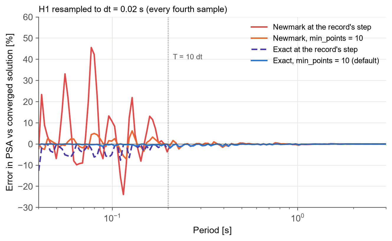
Newmark at the record's own step is off by up to about 45% at short periods, and even the exact solver under-reads the peaks by up to 12%. With the default settings, exact solver and min_points = 10, the error disappears. Above 10 time steps (0.2 s here), all options agree.
sig.Component(acc1, dt, solver="newmark")   # Newmark instead of exact
sig.Component(acc1, dt, min_points=None)    # solve at the record's own step
sig.Component(acc1, dt, precision=64)       # double precision throughout

# The solvers are also available directly, returning full response histories
u, v, a = sig.nigam_jennings(acc1, dt, [0.5, 1.0], xi=0.05)
u, v, a = sig.lrha(acc1 * sig.GRAVITY, dt, [0.5, 1.0], 0.05)
Conditioning a record
Raw records often carry a drift in the baseline and noise at very low and very high frequencies. Two tools are provided:
- Baseline correction removes a constant, linear, quadratic or cubic trend fitted to the record.
- Butterworth filtering in low-pass, high-pass, band-pass or band-stop form, causal (one pass) or acausal (zero phase). The record is tapered and padded before filtering, following Boore and Akkar (2003) and Boore (2005).
Both return a new Component or GroundMotion with the same settings, so they chain naturally:
h1.baseline_corrected("Linear")
h1.filtered(cut_off=(0.1, 25), filter_order=4)                  # band-pass, acausal
pair.baseline_corrected("Linear").filtered(cut_off=(0.1, 25))   # both components

# The same operations on plain arrays
sig.baseline_correction(acc1, dt, "Quadratic")
sig.butterworth_filter(acc1, dt, cut_off=0.1, filter_type="highpass")
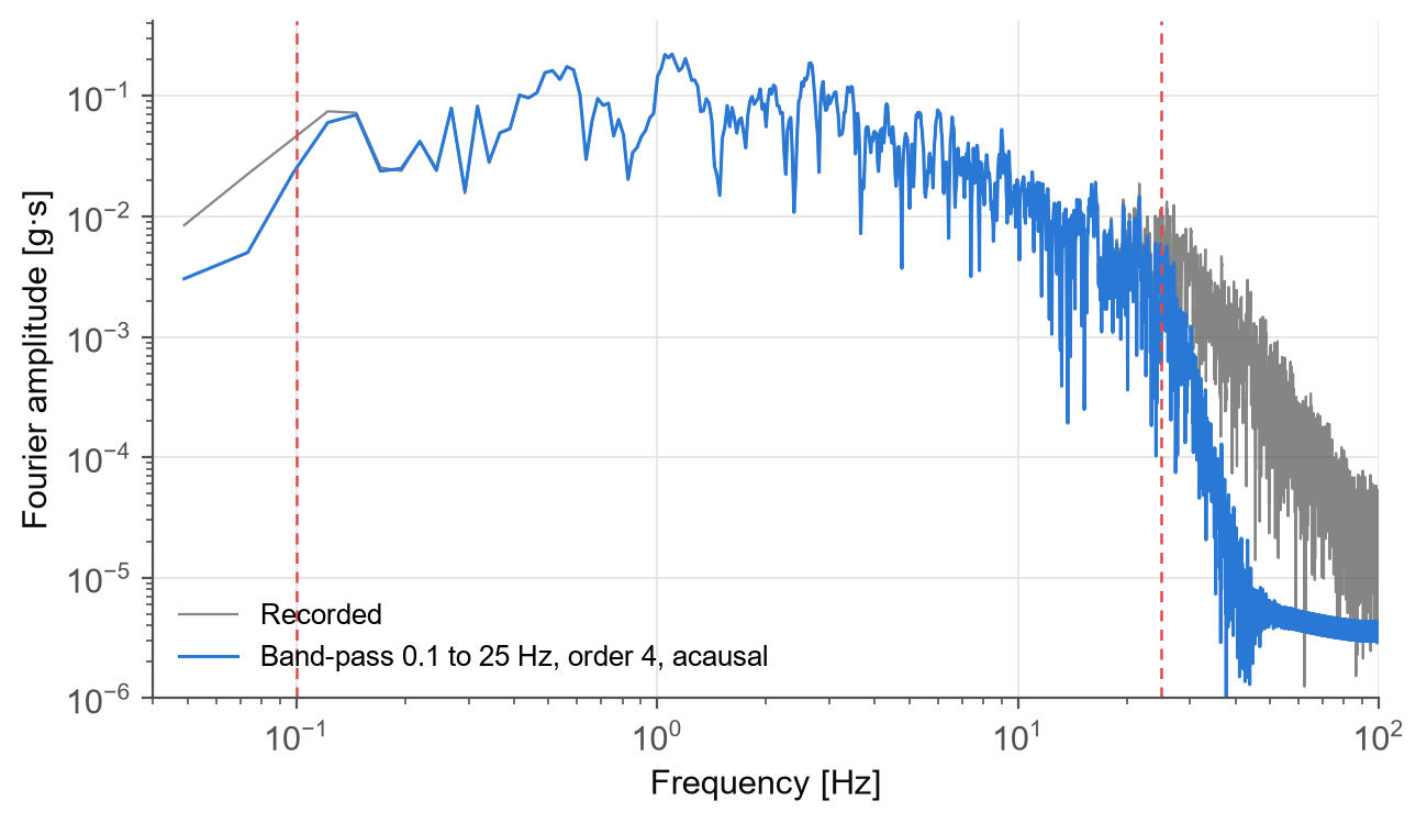
The record used here has already been processed by PEER, so filtering it again at 0.1 to 25 Hz mainly removes the content above 25 Hz. For raw records, the choice of corner frequencies deserves care, since it controls the long-period content and therefore the displacement.
Near-fault pulses
Records close to a fault can contain a strong, long-period velocity pulse, caused by rupture directivity. Pulses impose large demands on flexible structures, so identifying them matters both for record selection and for hazard analysis.
The module implements the classifier of Shahi and Baker (2014), building on Baker (2007). It uses a wavelet transform to search both horizontal components for the strongest pulse, in any direction. It then extracts the pulse, computes what remains, and decides whether the record is pulse-like.
pair.tpulse           # 4.79 s; -999 if no pulse is found
pair.pulse.make_plot()
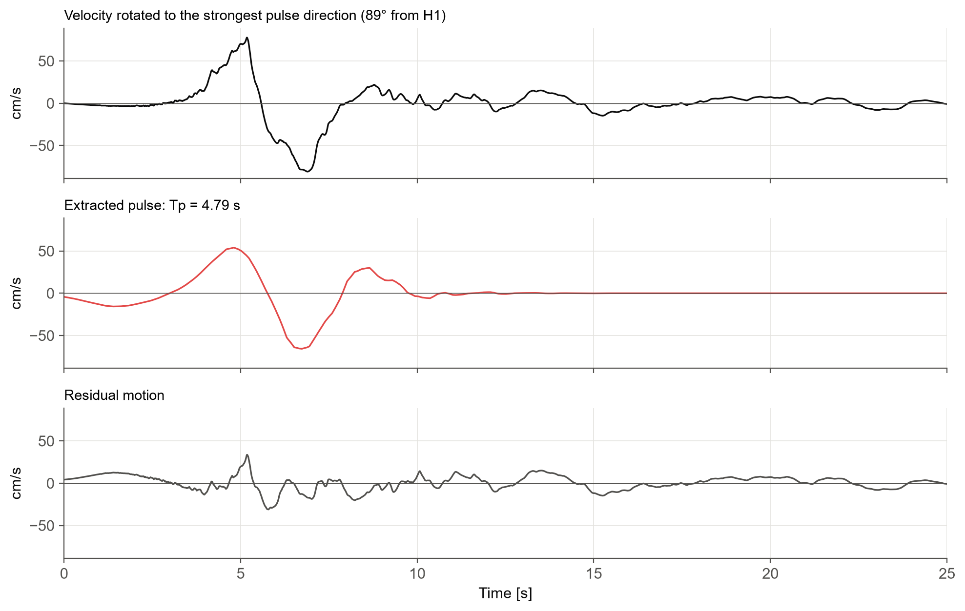
El Centro Array #4 is classified as pulse-like, with a pulse period of 4.79 s. The strongest pulse lies almost at right angles to H1, close to the H2 component that showed the large velocity swing at the start of this post. Removing the pulse brings the peak velocity down from 81 cm/s to 34 cm/s: most of the velocity in this record is the pulse.
Every measure at a glance
All measures are returned in conventional units, listed in sig.IM_UNITS. The table below summarises what is available on a Component; every one of them can also be rotated with GroundMotion.rotd.
| Group | Measures | Units |
|---|---|---|
| Peaks | pga, pgv, pgd | g, cm/s, cm |
| Energy and amplitude | ia, cav, arms, vrms, drms, ic | m/s, g·s, g, cm/s, cm, - |
| Duration | ds575, ds595, significant_duration, bracketed_duration, uniform_duration | s |
| Frequency content | fas, pas, tm | g·s, -, s |
| Response spectra | psa, psv, sd, sa_rel, sv_rel, sa_abs, sv_abs, sd_abs, tp | g, cm/s, cm, s |
| Spectrum intensities | si, asi, masi, dsi | cm, g·s, g·s, cm·s |
| Input energy | ei_rel, ei_abs, v_eq | m²/s², m²/s², cm/s |
| Next-generation | sa_avg, fiv3 | g, cm/s |
| Pair only | rotd, geomean, at_angle, tpulse | as the measure, s |
Conclusion
Summary
This post went through every part of the signal_processing module using one real near-fault record.
We started with the time histories and their peaks, then summarised the whole record through Arias intensity, CAV, RMS values and the different duration definitions. The Fourier spectrum and mean period described its frequency content.
Response spectra showed how structures of different periods respond, with the pseudo- and true spectra, spectrum intensities over period bands, and input energy. Two next-generation IMs, Saavg and FIV3, captured more of the record than Sa at a single period.
For the two horizontal components, RotDxx gave orientation-independent values of any measure. The exact SDOF solver with automatic resampling kept the spectra accurate even for coarsely sampled records. Baseline correction and filtering condition raw records, and the pulse classifier identified the 4.8 s velocity pulse in this record.
All of it comes from two objects, Component and GroundMotion, with every measure one attribute or method away.
Try it yourself
The module is part of the open-source djura Python package:
pip install "djura[signal_processing]"
The record used here is in the package's test folder, so every number in this post can be reproduced.
Further reading
- Converting seismic fragility and vulnerability models between intensity measures: how the choice of PGA, Sa(T), Saavg(T) or FIV3(T) affects fragility models and average annual loss.
- Conditional spectrum record selection for multiple stripe analysis: selecting hazard-consistent ground motions with the generalised conditional spectrum method, including Saavg and FIV3.
- Unconditional record selection for rupture scenarios: selecting records for earthquake scenarios using IMs such as PGV, duration and FIV3.
- Hazard consistency of a selected ground motion record suite: checking selected records against the site hazard.
Stay Tuned
Get in touch if you would like to use this service, or see our risk engineering consulting services. Stay tuned for more posts, and contact us for more information.
Frequently asked questions
How do you compute a response spectrum from a ground motion record in Python?
With the djura package, create a Component from the acceleration and time step and call psa(periods) for the pseudo-spectral acceleration, or psv and sd for the other spectra. The default exact solver of Nigam and Jennings (1969) uses 5% damping and resamples the record at short periods so the peaks are not missed.
What is RotD50?
RotD50 is an orientation-independent measure of a two-component record: the pair is rotated through every angle from 0° to 180°, the measure is computed in each direction, and the median over all angles is taken. RotD100 is the maximum over all angles.
What is the difference between pseudo-spectral acceleration and true absolute acceleration?
Pseudo-spectral acceleration is PSA = ω²·Sd, which is what design codes, ground motion models and record selection mean by Sa(T). The true absolute acceleration is the actual peak acceleration of the oscillator; at 5% damping the two are almost identical.
How is average spectral acceleration Sa_avg computed?
Sa_avg(T) is the geometric mean of Sa over a range of periods around T. By default the djura module averages 10 periods from 0.2T to 2.0T, and both bounds and the number of periods can be changed.
How can I detect a velocity pulse in a ground motion record?
The djura module implements the Shahi and Baker (2014) classifier, which uses a wavelet transform to search both horizontal components for the strongest pulse in any direction. For El Centro Array #4 (RSN 179) it finds a pulse with a period of 4.79 s.
References
- Arias A (1970) A measure of earthquake intensity. In: Seismic Design for Nuclear Power Plants. MIT Press, 438–483.
- Baker JW (2007) Quantitative classification of near-fault ground motions using wavelet analysis. Bulletin of the Seismological Society of America 97(5): 1486–1501.
- Baker JW, Cornell CA (2006) Spectral shape, epsilon and record selection. Earthquake Engineering & Structural Dynamics 35(9): 1077–1095.
- Boore DM (2005) On pads and filters: processing strong-motion data. Bulletin of the Seismological Society of America 95(2): 745–750.
- Boore DM (2010) Orientation-independent, nongeometric-mean measures of seismic intensity from two horizontal components of motion. Bulletin of the Seismological Society of America 100(4): 1830–1835.
- Boore DM, Akkar S (2003) Effect of causal and acausal filters on elastic and inelastic response spectra. Earthquake Engineering & Structural Dynamics 32: 1729–1748.
- Bradley BA (2011) Empirical equations for the prediction of displacement spectrum intensity and its correlation with other intensity measures. Soil Dynamics and Earthquake Engineering 31(8): 1182–1191.
- Dávalos H, Miranda E (2019) Filtered incremental velocity: A novel approach in intensity measures for seismic collapse estimation. Earthquake Engineering & Structural Dynamics 48(12): 1384–1405.
- Housner GW (1952) Spectrum intensities of strong-motion earthquakes. Proceedings of the Symposium on Earthquake and Blast Effects on Structures, EERI, 20–36.
- Newmark NM (1959) A method of computation for structural dynamics. Journal of the Engineering Mechanics Division 85(3): 67–94.
- Nigam NC, Jennings PC (1969) Calculation of response spectra from strong-motion earthquake records. Bulletin of the Seismological Society of America 59(2): 909–922.
- Rathje EM, Abrahamson NA, Bray JD (1998) Simplified frequency content estimates of earthquake ground motions. Journal of Geotechnical and Geoenvironmental Engineering 124(2): 150–159.
- Shahi SK, Baker JW (2014) An efficient algorithm to identify strong velocity pulses in multi-component ground motions. Bulletin of the Seismological Society of America 104(5): 2456–2466.
- Trifunac MD, Brady AG (1975) A study on the duration of strong earthquake ground motion. Bulletin of the Seismological Society of America 65(3): 581–626.
- Uang CM, Bertero VV (1990) Evaluation of seismic energy in structures. Earthquake Engineering & Structural Dynamics 19(1): 77–90.
- Von Thun JL, Roehm LH, Scott GA, Wilson JA (1988) Earthquake ground motions for design and analysis of dams. Earthquake Engineering and Soil Dynamics II, ASCE, 463–481.
- Shahnazaryan D, Ozsarac V, O'Reilly GJ (2025) Djura Ground Motion Record Selector: A Software Solution for Earthquake Engineering. COMPDYN 2025, Rhodes, Greece. DOI: 10.7712/120125.12444.25126