Conditional Spectrum Record Selection Explained
What is the conditional spectrum?
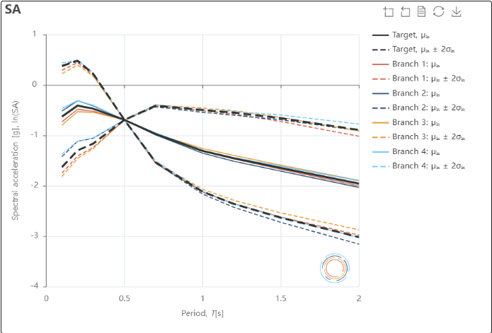
The conditional spectrum (CS) is the distribution of spectral accelerations at all periods that is expected at a site, given that spectral acceleration at one conditioning period, Sa(T*), equals a target value obtained from probabilistic seismic hazard analysis.
It is the basis of one of the most widely used approaches to ground motion record selection for nonlinear time-history analysis (Lin et al. 2013; Baker and Lee 2018). The core idea is simple: the selected ground motions have a known value of a conditioning intensity measure (IM), and every other IM of the records should then follow the distribution that the hazard implies for that value.
Why not just use a uniform hazard spectrum?
A uniform hazard spectrum (UHS) is built by reading, at each period, the spectral acceleration with the same exceedance probability from the site's hazard curves. Each ordinate is a valid hazard result on its own, but the spectrum as a whole is an envelope: the different periods are typically controlled by different earthquakes, and a single real ground motion is unlikely to reach the UHS at every period at once. Matching records to a UHS therefore tends to produce ground motions that are, overall, stronger than the hazard they are meant to represent.
UHS-based selection remains the basis of most building codes, and our tutorial on code-based record selection with a uniform hazard spectrum shows how to use it. The CS is the hazard-consistent alternative used when a site-specific probabilistic assessment is the goal.
How is a conditional spectrum built?
Building the target takes four ingredients: the hazard curve, the disaggregation, ground motion models and a correlation model.
- Choose the conditioning IM and its value. Typically Sa(T*), with T* a period relevant to the structure. Its target value, the conditioning value, is read from the site's hazard curve at the return period of interest.
- Find the earthquakes that cause it. The hazard disaggregation gives the rupture scenarios (magnitude, distance and other parameters) that contribute to exceeding that value.
- Measure how unusual the target is. For each scenario, a GMM gives the mean and standard deviation of ln Sa(T*). The number of standard deviations by which the target exceeds the mean is called epsilon, ε.
- Spread it to other periods. A correlation model gives how strongly an above-average Sa(T*) implies an above-average Sa at every other period. The result is a conditional mean and standard deviation at each period.
For a single scenario and a single GMM, the standard equations are:
Here and are the GMM's mean and standard deviation for a scenario of magnitude M and distance R, and is the correlation between the two spectral accelerations. At the conditioning period itself, ρ = 1, so the conditional standard deviation is zero: every selected record matches the target exactly there.
The conditional mean alone is known as the conditional mean spectrum (CMS). The CS adds the conditional standard deviation, so that the selected records reproduce the spread of spectral shapes as well as the average.
Approximate and exact conditioning
In practice, the disaggregation contains many rupture scenarios and the hazard model uses several GMMs. Using only the single dominant scenario is known as approximate conditional selection (Lin et al. 2013). Weighting every contributing scenario by its contribution to the hazard is called exact conditional selection, and gives a more accurate target. Several GMMs can also be combined with logic-tree weights, as is done in the hazard analysis itself. The difference between the two is one of the factors that decides whether the final record set is hazard-consistent.
Beyond spectral acceleration: the generalised conditional IM approach
Spectral acceleration does not describe everything about a ground motion. Two records with the same spectrum can differ in duration, velocity or cumulative energy, and those can matter for structural response.
The generalised conditional intensity measure (GCIM) approach (Bradley 2010) applies the same conditioning to any IM that has a GMM and a correlation model: significant duration, PGV, or next-generation IMs such as average spectral acceleration, Saavg(T) (Vamvatsikos and Cornell 2005; Eads et al. 2015), and filtered incremental velocity, FIV3(T) (Dávalos and Miranda 2019). The conditioning IM itself need not be Sa(T*) either. If you are new to FIV3, see what FIV3 (filtered incremental velocity) is and why it is so efficient.
From a target to a record set
Once the target exists, records are selected and amplitude-scaled from a ground motion database so that, together, they match the target distributions. The quality of the match can be checked statistically, for example by comparing the empirical distribution of the selected records with the target and its Kolmogorov-Smirnov limits. Baker and Lee (2018) describe an improved algorithm for selecting ground motions to match a conditional spectrum.
Multiple stripe analysis
A CS describes one intensity level. Repeating the selection at several return periods gives one record set, or stripe, per level. Running the structure under every stripe is multiple stripe analysis (MSA) (Jalayer and Cornell 2009), and fitting the fraction of records that exceed a damage state at each stripe gives a fragility function. For a refresher on what such a function represents, see what a fragility curve is.
This is exactly how the reference models were built in our study on converting fragility models between intensity measures: ground motions were selected with the conditional spectrum method through the Djura record selector, 40 records per intensity level, and multiple stripe analysis gave fragility functions in 18 IMs. The conversion method in that study also relies on the same conditional distribution of one IM given another that CS record selection uses.
Is the record set hazard-consistent?
A record set is hazard-consistent when the hazard curves implied by the selected records, for IMs other than the conditioning one, agree with the hazard curves from PSHA (Lin et al. 2013). When they do, risk estimates stay consistent whichever conditioning period is chosen. Approximate rather than exact conditioning, the assumption that correlation models are independent of the rupture and ground motion models, and the residual mismatch between the selected records and the target can all erode it. Our post on checking the hazard consistency of a selected record suite shows how to verify it.
Selecting conditional spectrum records with Djura
The Djura record selector (Shahnazaryan et al. 2025) implements generalised conditional selection with:
- multiple rupture scenarios, weighted by their contribution to the hazard, for exact conditioning;
- multiple GMMs per IM, with user-defined weights;
- non-spectral and next-generation IMs, including duration, PGV, Saavg and FIV3;
- a choice of horizontal component definition (geomean, RotD50 or RotD100), scaling limits, and limits on causal parameters such as magnitude or faulting style.
The target distributions use the correlation models of Aristeidou et al. Our step-by-step conditional spectrum record selection tutorial walks through every screen, from defining IM-GMM pairs and rupture scenarios to downloading the scaled records. For selection for a given earthquake scenario rather than a hazard level, see the scenario-based record selection tutorial.
Frequently asked questions
What is the difference between the conditional mean spectrum and the conditional spectrum?
The conditional mean spectrum (CMS) is the mean spectral acceleration at every period given the target value at the conditioning period. The conditional spectrum (CS) adds the conditional standard deviation, so that the selected records also reproduce the expected spread of spectral shapes.
Why is conditional spectrum selection preferred over the uniform hazard spectrum?
A uniform hazard spectrum envelopes the contributions of different earthquakes across periods, so a single ground motion is unlikely to match it everywhere. The conditional spectrum represents the shaking expected at a site given one target intensity, which supports hazard-consistent record selection.
What is the difference between approximate and exact conditional selection?
Approximate conditional selection builds the target from a single dominant rupture scenario. Exact conditional selection weights every contributing rupture scenario by its contribution to the hazard, as given by the disaggregation.
References
- Lin T, Haselton CB, Baker JW (2013) Conditional spectrum-based ground motion selection. Part I: Hazard consistency for risk-based assessments. Earthquake Engineering & Structural Dynamics 42(12): 1847–1865. doi:10.1002/eqe.2301
- Baker JW, Lee C (2018) An Improved Algorithm for Selecting Ground Motions to Match a Conditional Spectrum. Journal of Earthquake Engineering 22(4): 708–723. doi:10.1080/13632469.2016.1264334
- Jalayer F, Cornell CA (2009) Alternative non-linear demand estimation methods for probability-based seismic assessments. Earthquake Engineering & Structural Dynamics 38(8): 951–972. doi:10.1002/eqe.876
- Bradley BA (2010) A generalized conditional intensity measure approach and holistic ground-motion selection. Earthquake Engineering & Structural Dynamics 39(2): 1321–1342. doi:10.1002/eqe.995
- Vamvatsikos D, Cornell CA (2005) Developing efficient scalar and vector intensity measures for IDA capacity estimation by incorporating elastic spectral shape information. Earthquake Engineering & Structural Dynamics 34(13): 1573–1600. doi:10.1002/eqe.496
- Eads L, Miranda E, Lignos DG (2015) Average spectral acceleration as an intensity measure for collapse risk assessment. Earthquake Engineering & Structural Dynamics 44(12): 2057–2073. doi:10.1002/eqe.2575
- Dávalos H, Miranda E (2019) Filtered incremental velocity: A novel approach in intensity measures for seismic collapse estimation. Earthquake Engineering & Structural Dynamics 48(12): 1384–1405. doi:10.1002/eqe.3205
- Aristeidou S, Shahnazaryan D, O'Reilly GJ (2025) Correlation models for next-generation amplitude and cumulative intensity measures using artificial neural networks. Earthquake Spectra 41(1): 851–875. doi:10.1177/87552930241270563
- O'Reilly GJ, Ozsarac V, Shahnazaryan D (2026) Conversion of Seismic Fragility and Vulnerability Models to Alternative Intensity Measures for Regional Risk Analysis. Earthquake Spectra 42: e70098. doi:10.1002/esp4.70098
- Shahnazaryan D, Ozsarac V, O'Reilly GJ (2025) Djura Ground Motion Record Selector: A Software Solution for Earthquake Engineering. COMPDYN 2025, Rhodes, Greece. doi:10.7712/120125.12444.25126