Exact Conditional Spectrum-Based Record Selection
- Background
- Worked example with the Python package CODE
- When to use the exact approach
- Reproducing this post

Any PSHA software: describe the hazard in input.json
A conditional spectrum target needs three ingredients: the scenarios that cause the hazard, the GMMs that predict ground motion for those scenarios, and the correlation between intensity measures. If you are new to the method, Conditional Spectrum Record Selection Explained covers the theory, and the record selector post shows the web app.
The open-source djura Python package, released under the AGPL-3.0 licence and installed with pip install "djura[record_selection]", does not tie these ingredients to a particular hazard code. Its GCIM record selector reads them from a single input.json, so in principle any PSHA software can drive it. You describe the GMMs, the site, the rupture scenarios with their weights, and the conditioning intensity measure IM* with its value from the hazard curve:
{
  "gmms": [
    // Active Shallow Crust GMMs
    {"ID": 0, "SA": {"names": ["BooreAtkinson2008", "ChiouYoungs2008"], "weights": [0.6, 0.4]}},
    // Stable Continental Crust GMMs
    {"ID": 1, "SA": {"names": ["AtkinsonBoore2006", "Atkinson2008prime"], "weights": [0.7, 0.3]}}
  ],
  "site-parameters": {"vs30": 600, "z1pt0": 100},
  "ruptures": [
    // Active Shallow Crust rupture
    {"mag": 6.3, "rjb": 10, "rrup": 12, "rx": 120, "ztor": 0, "weight": 0.6, "gmms": [0]},
    // Stable Continental Crust rupture
    {"mag": 6.0, "rjb": 20, "rrup": 20, "rx": 120, "ztor": 0, "weight": 0.4, "gmms": [1]}
  ],
  // Intensity measures to match
  "imi": ["SA(0.1)", "SA(0.2)", "SA(0.5)", "SA(1.0)", "SA(2.0)"],
  // Conditioning intensity measure and its value, IM*
  "im-star": {"type": "SA(0.5)", "value": 0.189},
  "num_records": 40,
  "max_scaling_factor": 3
}
The comments are for illustration only; JSON does not allow them, so leave them out of a real file. Each rupture lists the GMM groups that apply to it. A rupture from an active shallow crust source is evaluated with the active shallow GMMs only, and a stable continental one with its own. This is how a logic tree over several tectonic region types (TRTs) is expressed.
The weak point is the ruptures block. Most hazard software exports a disaggregation, a table of magnitude-distance(-epsilon) bins, and each bin becomes one scenario at its bin centre. The other parameters the GMMs need, such as Rx, Ztor, dip and rake, have to be borrowed from a nearby rupture or assumed. This approximate input works well and runs in the Djura web app. Every simplification, however, moves the target a little away from the hazard it is meant to represent.
Using OpenQuake's datastore for target generation
If the PSHA was run in the OpenQuake Engine, there is no need to approximate. The engine keeps every rupture it considered, with the exact parameters it passed to the GMMs, in its calculation datastore.
Every OpenQuake calculation writes its inputs, intermediate results and outputs to a single HDF5 file, the datastore. It is named calc_<id>.hdf5, after the calculation ID, and sits in the engine's data directory: ~/oqdata on Linux and macOS, C:\Users\<you>\oqdata on Windows, or wherever OQ_DATADIR points. The exported CSV and XML outputs are only views of it; the datastore is the complete record of the run.
For record selection, these are the parts that matter:
| Datastore content | Why record selection needs it |
|---|---|
| Rupture contexts, grouped by source group | Magnitude, every distance metric, rake, dip, Ztor and the occurrence rate of each rupture, exactly as passed to the GMMs |
| Context makers and GMMs per group | Which GMMs apply to which ruptures, and the parameters each GMM requires |
| Logic tree and realisation weights | The weight each group-GMM pair carries |
| Site collection | Vs30, Z1.0 and the other site parameters of the run |
| Hazard curves | The value of IM* at the target PoE |
| Job parameters | Investigation time, truncation level, intensity measures and PoEs |
Not every calculation stores the rupture contexts. A disaggregation run (calculation_mode = disaggregation), as in the example below, always does. A datastore is also tied to the engine version that wrote it, so read it with the same version.
djura-tools, the open-source companion repository of djura, also under AGPL-3.0, reads that datastore and hands the whole PSHA to the record selector. We call this the exact approach.
Approximate (input.json) | Exact (OpenQuake datastore) | |
|---|---|---|
| Hazard input | Disaggregation from any PSHA software | The datastore, calc_<id>.hdf5 |
| Scenarios | One per magnitude-distance bin | Every rupture of the PSHA |
| Rupture parameters | Bin centre, rest matched or assumed | The engine's own rupture contexts |
| GMMs and site | Written by hand | Read from the datastore |
| Weights | Hazard contribution of the bin | Logic-tree leaf weight × the rupture's rate of exceeding IM* (or of occurring at it) |
| Computational cost | Set by the number of bins, small for any model size | Grows with the number of ruptures and logic-tree realisations |
| Needs | djura | djura + djura-tools + the openquake.engine package |
| Web app | Yes | Python API only |
How the ruptures are weighted
Every rupture of the PSHA is evaluated with every GMM of its source group, and each rupture-GMM pair receives a weight. Three quantities enter it:
- The logic-tree weight of the GMM within the rupture's source group: the source-model weight times the GMM weight, as worked out for the example below.
- The annual rate of the rupture, , where is the probability that it occurs at least once in the investigation time .
- The epsilon of the conditioning level, , where and are the mean and standard deviation of ln IM* that GMM predicts for rupture . It measures how unusual is for that pair.
The two forms differ only in how is turned into a contribution.
Exceedance (default). Following Lin et al. (2013), each pair is weighted by its rate of producing IM* above :
where is the probability that IM* exceeds , from the normal distribution truncated at , the truncation level of the run, and is the standard normal cumulative distribution function. Summed over all pairs, the numerator is the total rate of exceeding , which is the hazard curve at the target PoE, .
Occurrence. Each pair is weighted by its rate of producing IM* at . Differentiating the exceedance probability with respect to the IM level turns it into a probability density. The probability of occurrence, IM* falling in a narrow band around , is that density times the width of the band; the width is the same for every pair and cancels in the normalisation, so the weights follow from the density:
where is the standard normal density, and is zero beyond the truncation level. The division by converts the density of ε into a density of ln IM*, so pairs with different standard deviations are compared on the same scale.
Exceedance or occurrence?
The conditional spectrum is conditioned on IM* being equal to : the ε of every pair is evaluated at itself. The exceedance weights, however, count each pair by how often it produces motions anywhere above , which favours pairs for which is easily exceeded. Fox et al. (2016) showed that the weights consistent with conditioning on come from the occurrence form. djura uses exceedance by default, as is common practice, and occurrence with one setting, shown in Step 2 below; both are computed from the same ruptures and GMMs.
The hazard model of the example
The example is Example 2 of the djura documentation. Its job file, source models, GMM logic tree and the resulting datastore are all in tests/rs/exact of the djura repository. It is a small synthetic model with a non-trivial logic tree, chosen because the logic tree is what the exact approach has to get right.
The site is at longitude 0.5, latitude -0.5, with Vs30 = 600 m/s (measured), Z1.0 = 100 m and Z2.5 = 5 km. Hazard curves were computed for 22 intensity measures (PGA, SA(0.05 s), and SA(0.1 s) to SA(2.0 s) in steps of 0.1 s) over an investigation time of 50 years, and disaggregated at a PoE of 10%, with a maximum distance of 200 km and GMM truncation at 3σ.
Source-model logic tree
Three source models, each with area and fault sources in two TRTs:
| Branch | Source model | Weight |
|---|---|---|
b1 | source_model_1.xml | 0.5 |
b2 | source_model_2.xml | 0.3 |
b3 | source_model_3.xml | 0.2 |
GMM logic tree
Each TRT has its own GMM branch set, so a source only ever sees the GMMs of its own TRT:
| Tectonic region type | GMM | Weight |
|---|---|---|
| Active Shallow Crust | BooreAtkinson2008 | 0.6 |
| Active Shallow Crust | ChiouYoungs2008 | 0.4 |
| Stable Continental Crust | AtkinsonBoore2006 | 0.7 |
| Stable Continental Crust | Atkinson2008prime | 0.3 |
The full logic tree
The engine enumerates every path through the tree, source model first, then the Active Shallow Crust GMM, then the Stable Continental Crust GMM. That gives 3 × 2 × 2 = 12 realisations, each weighted by the product of its branch weights:
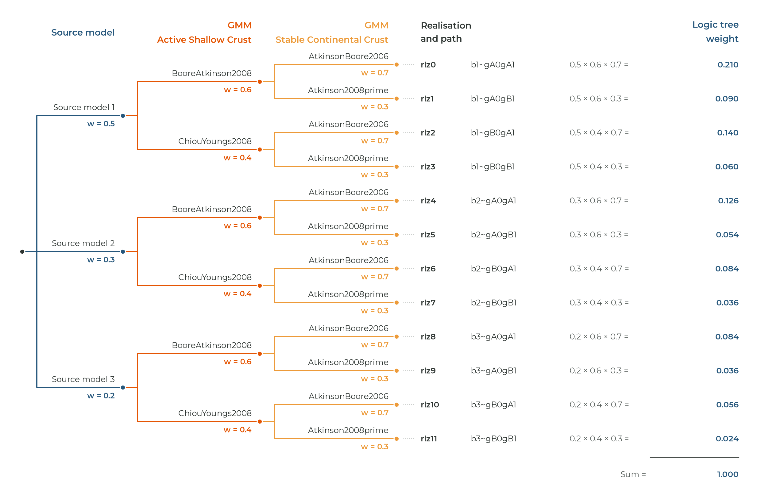
The path names are OpenQuake's. The source-model branch keeps its ID (b1 to b3), while the GMM branches are renamed with a letter per branch and a digit per TRT: gA0 and gB0 are BooreAtkinson2008 and ChiouYoungs2008 on TRT 0, Active Shallow Crust; gA1 and gB1 are AtkinsonBoore2006 and Atkinson2008prime on TRT 1, Stable Continental Crust. The weights range from 0.210 for b1~gA0gA1 down to 0.024 for b3~gB0gB1. They are stored in the datastore and read by djura-tools as ctx["lt-weights"].
Internally, OpenQuake does not compute each realisation separately. It splits the sources into 6 source groups, one per source model and TRT, holding 23,016 ruptures in total, and evaluates each group under the two GMMs of its TRT. A rupture in an Active Shallow Crust group is never evaluated with a Stable Continental GMM, so for that rupture the Stable Continental branch makes no difference. Its weight under a GMM is therefore the sum of the realisations that share that source model and GMM, which reduces to the source-model weight times the GMM weight. For BooreAtkinson2008 in source model 1, rlz0 + rlz1 = 0.210 + 0.090 = 0.30 = 0.5 × 0.6. These 12 group-GMM weights, ctx["gsim-weights"], are the in the weight equations above:
| Group | Source model | TRT | Ruptures | GMM weights (= source model × GMM) |
|---|---|---|---|---|
| 0 | b1 | Active Shallow Crust | 1,334 | BooreAtkinson2008 0.30, ChiouYoungs2008 0.20 |
| 1 | b2 | Active Shallow Crust | 1,297 | BooreAtkinson2008 0.18, ChiouYoungs2008 0.12 |
| 2 | b3 | Active Shallow Crust | 2,165 | BooreAtkinson2008 0.12, ChiouYoungs2008 0.08 |
| 3 | b1 | Stable Continental Crust | 4,100 | AtkinsonBoore2006 0.35, Atkinson2008prime 0.15 |
| 4 | b2 | Stable Continental Crust | 5,920 | AtkinsonBoore2006 0.21, Atkinson2008prime 0.09 |
| 5 | b3 | Stable Continental Crust | 8,200 | AtkinsonBoore2006 0.14, Atkinson2008prime 0.06 |
The weights of the three Active Shallow groups add up to 1, and so do those of the three Stable Continental ones, because every realisation contains exactly one group of each TRT. Writing 23,016 ruptures and these weights into input.json by hand is not realistic; reading them from the datastore is.
Step 1: extract the disaggregation context with djura-tools
djura has no dependency on OpenQuake. The datastore reader, get_context_from_dstore, lives in djura-tools and opens the file through the OpenQuake Python API. It therefore runs in an environment with the openquake.engine package installed. No calculation is run; the package is only used to read the file.
pip install openquake.engine
git clone https://github.com/djura-risk-data-engineering/djura-tools
cd djura-tools
From that clone:
import pickle
from djura.hazard.dstore import get_context_from_dstore

# im_ref is the IM the conditioning value is read in. It can be changed
# later on the returned dictionary without re-reading the datastore.
ctx, oq = get_context_from_dstore("calc_2.hdf5", im_ref="SA(0.5)")

with open("ctx_2.pickle", "wb") as f:
    pickle.dump(ctx, f)

print(ctx["totrups"], ctx["site-parameters"], ctx["required-parameters"])
# 23016 ['vs30', 'vs30measured', 'z1pt0']
# {'mag', 'rake', 'dip', 'ztor', 'rrup', 'rjb', 'rx'}
ctx is a plain dictionary that holds the hazard in the form djura needs. Once it is pickled, neither the datastore nor OpenQuake is needed again, and the pickle can be shared with anyone who runs the selection:
| Key | Content |
|---|---|
ctx_by_grp | One record array of rupture contexts per source group, six here |
required-parameters | The rupture and distance parameters the GMMs need, read from each rupture: mag, rake, dip, ztor, rrup, rjb, rx |
site-parameters | The site parameters the GMMs need: vs30, vs30measured, z1pt0 |
gsims, gsim-weights | The 12 group-GMM pairs and their weights |
lt-weights | The 12 realisation weights |
hazard-curves, imt, oq-poes | Hazard curves, IM levels and PoEs, which give the conditioning value |
invtime, phi_b | Investigation time (50 years) and the standard normal cumulative probability at the truncation level |
Step 2: select the records with djura
From here on only djura is needed, in any environment. The context replaces the hazard part of input.json: the GMMs, site parameters, ruptures, IM vector and conditioning value all come from it. What you still write are the selection settings.
import pickle

from djura.record_selection.gcim import GCIM

with open("ctx_2.pickle", "rb") as f:
    ctx = pickle.load(f)

# Condition on SA(0.5 s); any IM of the run can be used here
ctx["im_ref"] = "SA(0.5)"

settings = {
    "num_records": 40,
    "num-components": 2,
    "component-definition": "RotD50",
    "max_scaling_factor": 3.0,
    "nreplicate": 20,
    "correlation-models": {"SA-SA": "baker_jayaram"},
}

gcim = GCIM(settings, conditional=True, dis_oq=ctx, poe_for_selection=0.1)
target = gcim.create()
poe_for_selection must lie within the PoEs of the run, ctx["oq-poes"]. Here that is only 0.1, giving SA(0.5 s) = 0.189 g. create() builds the GCIM target from all 23,016 ruptures under their GMMs.
To weight the ruptures by occurrence instead of exceedance when building the target, add "occurrence": True to the selection settings. The datastore needs nothing extra, because the density is computed for every rupture from the same GMMs:
settings = {
    # ... the selection settings above
    "occurrence": True,   # weight ruptures by occurrence at IM*
}
gcim = GCIM(settings, conditional=True, dis_oq=ctx, poe_for_selection=0.1)
target = gcim.create()
For the example model, the two targets compare as follows at SA(0.5 s) = 0.189 g:
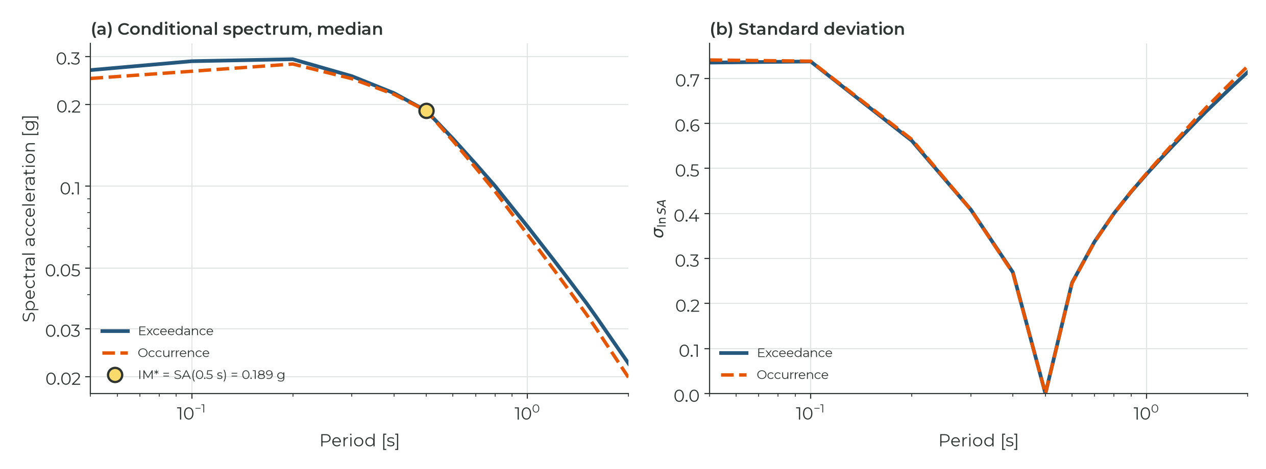
| T s | Exceedance g | Occurrence g | Difference |
|---|---|---|---|
| PGA | 0.174 | 0.170 | −2% |
| 0.1 | 0.288 | 0.265 | −8% |
| 0.2 | 0.293 | 0.281 | −4% |
| 0.5 | 0.189 | 0.189 | 0% |
| 1.0 | 0.071 | 0.067 | −7% |
| 2.0 | 0.022 | 0.020 | −11% |
Which intensity measures are matched
In the exact approach you do not choose the intensity measures to match. The IM vector is set to every intensity measure type of the OpenQuake run, that is, the keys of intensity_measure_types_and_levels in the job file, stored in ctx["imt"]. An imi entry in the settings is overridden. The reason is consistency: the conditioning value has to come from a hazard curve, and the target for each IM is built with the GMMs of the same logic tree, so the selection is limited to what the PSHA actually computed.
In this example that means 22 intensity measures:
- PGA,
- SA(0.05 s), and SA(0.1 s) to SA(2.0 s) in steps of 0.1 s, 21 spectral periods in total.
One of them, SA(0.5 s), is the conditioning IM chosen with ctx["im_ref"]. The other 21 get a full conditional distribution, a median and a standard deviation, which the records are fitted to. Each piece of that comparison has its own source:
| What | Where it comes from |
|---|---|
| The list of IMs | The job file, through ctx["imt"] |
| The value of IM* | The mean hazard curve of SA(0.5 s) in the datastore, ctx["hazard-curves"], read at the PoE given by poe_for_selection: 0.189 g at 10% in 50 years |
| The median and σ of each IM, per rupture | The GMMs of the rupture's source group (BooreAtkinson2008 and ChiouYoungs2008 for active shallow crust, AtkinsonBoore2006 and Atkinson2008prime for stable continental crust), evaluated by djura with the rupture's own context parameters |
| The conditioning on IM* | The correlation between each IM and SA(0.5 s): Baker and Jayaram (2008) for SA-SA pairs, as set in correlation-models, and Bradley (2011), the default, for PGA-SA |
| The combined target | All rupture-GMM pairs, weighted by exceedance or occurrence as in the equations above, combined into one distribution per IM following Bradley (2010) |
| The records' IMs | Pre-computed in the flatfile, columns SA_RotD50 and PGA_RotD50, at 111 periods that include all 21 used here, so no interpolation is needed |
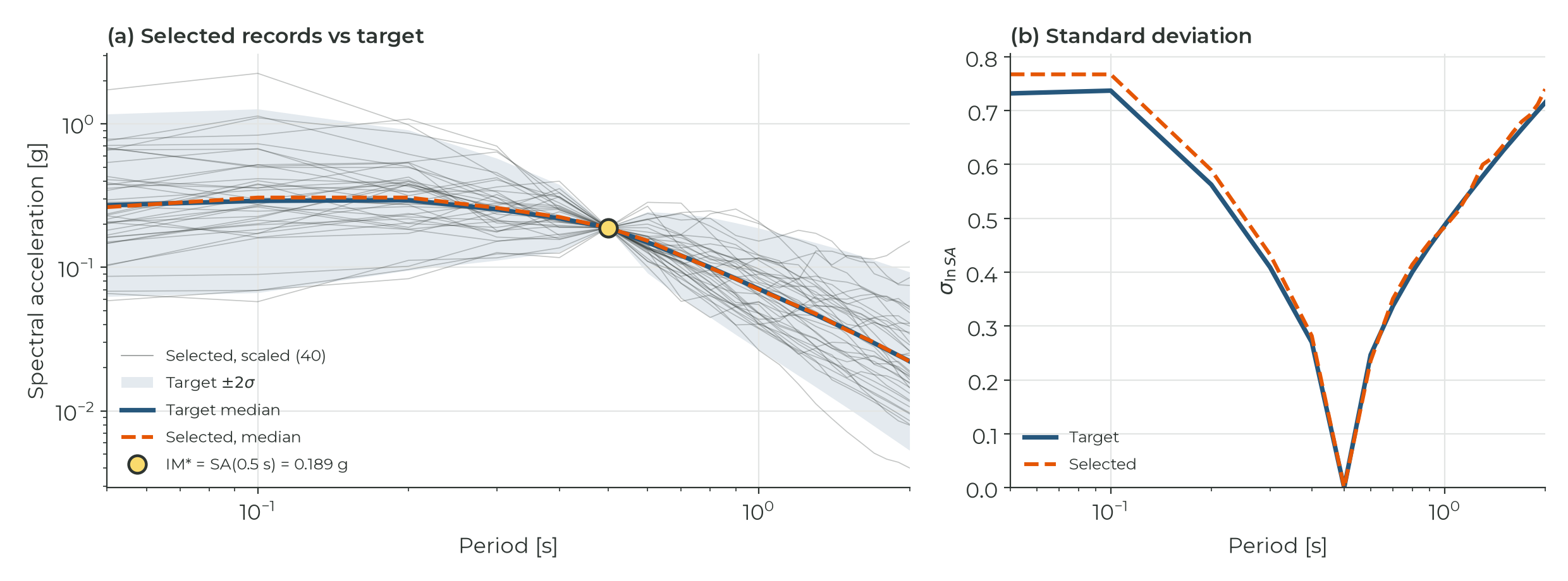
Both sides are compared in the same component definition, RotD50 of the two horizontal components, as set by component-definition. The GMMs predict that definition, and the flatfile stores it for every record. Each selected record is scaled by a single factor that brings its SA(0.5 s) to 0.189 g, and that factor applies to all 22 IMs. This is why all records pass through IM* in the figure under Running the selection.
To condition on another IM, change ctx["im_ref"] to any other entry of ctx["imt"]; no new PSHA run is needed. To match an IM that is not in the job file, such as PGV, a longer period or , add it to intensity_measure_types_and_levels, re-run the PSHA and extract the context again.
Running the selection
Records are selected from djura's default flatfile, which holds the 20,672 records of the European Strong Motion (ESM) database. Selection starts by simulating 40 spectra from the target distribution, which the records are then matched to one by one. nreplicate, set to 20 above, repeats the simulation and keeps the sample whose mean, standard deviation and skewness are closest to the target:
records = gcim.select()
select() picks 40 records from the 20,672 in the flatfile and scales them to the target. Together, create() and select() take about five minutes, most of it spent evaluating the GMMs for all 23,016 ruptures in create().
The figure below shows the result. The 40 records come from events of M3.9 to M7.7, with scale factors from 0.35 to 3.00, inside the limit of 3. The median of the selected set follows the target across all periods. Its standard deviation follows the target too, slightly above it at the shortest periods. The Kolmogorov-Smirnov check at α = 0.05 passed for PGA and every spectral period except SA(0.5 s). That is the conditioning IM: every record is scaled to exactly 0.189 g there, so the target has no spread and the test has nothing to compare.
Downloading the records from ESM
select() returns which records were chosen and their scale factors, not the waveforms. Since every record comes from ESM, the time histories can be fetched from the ESM web service with djura's ESMDownloader. It needs a free account at esm-db.eu.
ESM identifies a record by its event ID and the code of the recording station. Both are in the flatfile, at the indices select() returns under Rec_ID:
from djura.data_loader import get_metadata
from djura.record_selection import ESMDownloader

best = records["selected_scaled_best"]
metadata = get_metadata()
rec_ids = best["Rec_ID"]

events = metadata["esm_event_id"][rec_ids].tolist()
# Station_name is "<network>-<station>"; ESM expects the station code alone
stations = [name.split("-", 1)[1]
            for name in metadata["Station_name"][rec_ids]]

downloader = ESMDownloader(
    download_dir="records",
    events=events,
    stations=stations,
    username="example.user@email.com",  # your ESM account e-mail
    password="example.password",  # your ESM account password
)
zip_path = downloader.download()  # records/UnscaledRecords.zip
The two lists are paired element by element: the i-th record is the i-th event recorded at the i-th station. On the first call a token is requested with your credentials and saved as records/token.txt. Later runs can pass token_path instead of the credentials. Keep both the credentials and the token out of version control.
The 40 records arrive one request at a time and are collected into records/UnscaledRecords.zip, as the ASCII acceleration files served by ESM, one per component. As the name says, they are unscaled: multiply each time history by its factor in best["sf"], in the same order as Rec_ID, before running the analyses. A record the service does not serve is skipped rather than stopping the download. Skipped records are listed in downloader.failed_records and in records/FailedRecords.txt, and can be retried in a separate directory or replaced. The record downloader example in the djura documentation covers tokens, retries and errors in detail.
When to use the exact approach
The deciding factor is often the size of the hazard model. The exact approach evaluates the GMMs for every rupture of the PSHA, under every GMM its source group sees, at every intensity measure of the run. The work therefore grows with the number of ruptures and with the size of the logic tree: more source-model branches mean more copies of the ruptures, and more GMM branches mean more evaluations of each. The example here is deliberately small (23,016 ruptures, 12 realisations and 22 IMs), yet one selection already takes a few minutes. A regional or national model can carry millions of ruptures and hundreds or thousands of realisations. At that size the exact target becomes impractical to build, all the more so when it is repeated for several conditioning IMs and hazard levels, as in a multiple stripe analysis. A disaggregation condenses that same model into a few hundred magnitude-distance bins, whatever its size.
- Use
input.json, the approximate approach, when the hazard model is large, with many sources, ruptures or logic-tree realisations. Use it as well when the PSHA comes from software other than OpenQuake, when you want to work in the web app, or when the hazard is dominated by a few well-defined scenarios. - Use the OpenQuake datastore, the exact approach, when the model is small enough for every rupture to be evaluated in a reasonable time: a site-specific study, a limited maximum distance, or a modest logic tree. It pays off most when the GMMs depend on parameters such as Rx, Ztor or dip that disaggregation bins do not carry, or when you want a reference target to check an approximate one against.
Both routes build the target with the same GCIM code in djura. The only difference is where the ruptures and their weights come from, so a practical workflow is to build the exact target once for a representative case, confirm that the approximate one agrees with it, and then use the approximate approach for the full set of IMs and hazard levels.
Reproducing this post
Everything used here is open source under AGPL-3.0, and the example data ship with the djura repository:
- Hazard model and datastore: djura/tests/rs/exact, Example 2 (
assets/job_2.ini,assets/inputs_2/,data/calc_2.hdf5) - Datastore reader:
djura.hazard.dstore.get_context_from_dstorein djura-tools - Record selection and ESM download:
djura.record_selection.gcim.GCIManddjura.record_selection.ESMDownloaderin djura,pip install "djura[record_selection]"
The extracted context is bundled too, as data/ctx_2.pickle. With it you can skip Step 1 and run the selection with djura alone.
References
- Baker, J. W., and Jayaram, N. (2008). Correlation of spectral acceleration values from NGA ground motion models. Earthquake Spectra, 24(1), 299–317.
- Bradley, B. A. (2010). A generalized conditional intensity measure approach and holistic ground-motion selection. Earthquake Engineering & Structural Dynamics, 39(12), 1321–1342.
- Bradley, B. A. (2011). Empirical correlation of PGA, spectral accelerations and spectrum intensities from active shallow crustal earthquakes. Earthquake Engineering & Structural Dynamics, 40(15), 1707–1721.
- Fox, M. J., Stafford, P. J., and Sullivan, T. J. (2016). Seismic hazard disaggregation in performance-based earthquake engineering: occurrence or exceedance? Earthquake Engineering & Structural Dynamics, 45(5), 835–842.
- Lin, T., Harmsen, S. C., Baker, J. W., and Luco, N. (2013). Conditional spectrum computation incorporating multiple causal earthquakes and ground-motion prediction models. Bulletin of the Seismological Society of America, 103(2A), 1103–1116.
- Pagani, M., et al. (2014). OpenQuake Engine: an open hazard (and risk) software for the Global Earthquake Model. Seismological Research Letters, 85(3), 692–702.
- Shahnazaryan, D., Ozsarac, V., and O'Reilly, G. J. (2025). Djura ground motion record selector: a software solution for earthquake engineering. COMPDYN 2025. doi:10.7712/120125.12444.25126